Iterating Safely

Modern Plain Text Social Science
Week 07

Kieran Healy

kieran.healy@duke.edu

October 2026

Safely iterating with purrr and map

Load the packages, as always

library(here)      # manage file paths

here() starts at /Users/kjhealy/Documents/courses/mptc

library(socviz)    # data and some useful functions
library(tidyverse) # your friend and mine

── Attaching core tidyverse packages ──────────────────────── tidyverse 2.0.0 ──
✔ dplyr     1.2.1     ✔ readr     2.2.0
✔ forcats   1.0.1     ✔ stringr   1.6.0
✔ ggplot2   4.0.3     ✔ tibble    3.3.1
✔ lubridate 1.9.5     ✔ tidyr     1.3.2
✔ purrr     1.2.2     

── Conflicts ────────────────────────────────────────── tidyverse_conflicts() ──
✖ dplyr::filter() masks stats::filter()
✖ dplyr::lag()    masks stats::lag()
ℹ Use the conflicted package (<http://conflicted.r-lib.org/>) to force all conflicts to become errors

Additional libraries

library(survey)
library(srvyr)
library(broom)
library(gssr) # https://kjhealy.github.io/gssr

The complete GSS

data(gss_all)

gss_all

# A tibble: 75,699 × 6,942
   year         id wrkstat    hrs1        hrs2        evwork      occ   prestige
   <dbl+lbl> <dbl> <dbl+lbl>  <dbl+lbl>   <dbl+lbl>   <dbl+lbl>   <dbl> <dbl+lb>
 1 1972          1 1 [workin… NA(i) [iap] NA(i) [iap] NA(i) [iap] 205   50      
 2 1972          2 5 [retire… NA(i) [iap] NA(i) [iap]     1 [yes] 441   45      
 3 1972          3 2 [workin… NA(i) [iap] NA(i) [iap] NA(i) [iap] 270   44      
 4 1972          4 1 [workin… NA(i) [iap] NA(i) [iap] NA(i) [iap]   1   57      
 5 1972          5 7 [keepin… NA(i) [iap] NA(i) [iap]     1 [yes] 385   40      
 6 1972          6 1 [workin… NA(i) [iap] NA(i) [iap] NA(i) [iap] 281   49      
 7 1972          7 1 [workin… NA(i) [iap] NA(i) [iap] NA(i) [iap] 522   41      
 8 1972          8 1 [workin… NA(i) [iap] NA(i) [iap] NA(i) [iap] 314   36      
 9 1972          9 2 [workin… NA(i) [iap] NA(i) [iap] NA(i) [iap] 912   26      
10 1972         10 1 [workin… NA(i) [iap] NA(i) [iap] NA(i) [iap] 984   18      
# ℹ 75,689 more rows
# ℹ 6,934 more variables: wrkslf <dbl+lbl>, wrkgovt <dbl+lbl>,
#   commute <dbl+lbl>, industry <dbl+lbl>, occ80 <dbl+lbl>, prestg80 <dbl+lbl>,
#   indus80 <dbl+lbl>, indus07 <dbl+lbl>, occonet <dbl+lbl>, found <dbl+lbl>,
#   occ10 <dbl+lbl>, occindv <dbl+lbl>, occstatus <dbl+lbl>, occtag <dbl+lbl>,
#   prestg10 <dbl+lbl>, prestg105plus <dbl+lbl>, indus10 <dbl+lbl>,
#   indstatus <dbl+lbl>, indtag <dbl+lbl>, marital <dbl+lbl>, …

Set up our analysis

cont_vars <- c("year", "id", "ballot", "age")
cat_vars <- c("race", "sex", "fefam")
wt_vars <- c("vpsu",
             "vstrat",
             "oversamp",
             "formwt",              # weight to deal with experimental randomization
             "wtssall",             # main weight variable
             "sampcode",            # sampling error code
             "sample")              # sampling frame and method
my_vars <- c(cont_vars, cat_vars, wt_vars)

Clean the labeled variables

gss_df <- gss_all |>
  filter(year > 1974 & year < 2021) |>
  select(all_of(my_vars)) |>
  mutate(across(everything(), haven::zap_missing), # Convert labeled missing to regular NA
         across(all_of(wt_vars), as.numeric),
         across(all_of(cat_vars), as_factor),
         across(all_of(cat_vars), fct_relabel, tolower),
         across(all_of(cat_vars), fct_relabel, tools::toTitleCase),
         compwt = oversamp * formwt * wtssall)

Working dataset

gss_df

# A tibble: 60,213 × 15
   year         id ballot   age   race  sex   fefam  vpsu vstrat oversamp formwt
   <dbl+lbl> <dbl> <dbl+lb> <dbl> <fct> <fct> <fct> <dbl>  <dbl>    <dbl>  <dbl>
 1 1975          1 NA       38    White Male  <NA>      1   7001        1     NA
 2 1975          2 NA       20    White Fema… <NA>      1   7001        1     NA
 3 1975          3 NA       61    White Fema… <NA>      1   7001        1     NA
 4 1975          4 NA       19    White Male  <NA>      1   7001        1     NA
 5 1975          5 NA       28    White Male  <NA>      1   7001        1     NA
 6 1975          6 NA       28    White Fema… <NA>      1   7002        1     NA
 7 1975          7 NA       35    White Fema… <NA>      1   7002        1     NA
 8 1975          8 NA       64    White Fema… <NA>      1   7002        1     NA
 9 1975          9 NA       53    White Male  <NA>      1   7002        1     NA
10 1975         10 NA       34    White Fema… <NA>      1   7002        1     NA
# ℹ 60,203 more rows
# ℹ 4 more variables: wtssall <dbl>, sampcode <dbl>, sample <dbl>, compwt <dbl>

The fefam question

gss_df |>
  count(fefam)

# A tibble: 5 × 2
  fefam                 n
  <fct>             <int>
1 Strongly Agree     2543
2 Agree              8992
3 Disagree          13061
4 Strongly Disagree  5479
5 <NA>              30138

Recoding

gss_df <- gss_df |>
  mutate(fefam_d = forcats::fct_recode(fefam,
                                  Agree = "Strongly Agree",
                                  Disagree = "Strongly Disagree"),
    fefam_n = recode(fefam_d, "Agree" = 1, "Disagree" = 0))

# factor version
gss_df |>
  count(fefam_d)

# A tibble: 3 × 2
  fefam_d      n
  <fct>    <int>
1 Agree    11535
2 Disagree 18540
3 <NA>     30138

# numeric version, 1 is "Agree"
gss_df |>
  count(fefam_n)

# A tibble: 3 × 2
  fefam_n     n
    <dbl> <int>
1       0 18540
2       1 11535
3      NA 30138

Unweighted model

out_all <- glm(fefam_n ~ age + sex + race,
              data = gss_df,
              family="binomial",
              na.action = na.omit)

summary(out_all)

Call:
glm(formula = fefam_n ~ age + sex + race, family = "binomial", 
    data = gss_df, na.action = na.omit)

Coefficients:
              Estimate Std. Error z value Pr(>|z|)    
(Intercept) -1.9185878  0.0399581 -48.015  < 2e-16 ***
age          0.0323648  0.0007275  44.486  < 2e-16 ***
sexFemale   -0.2247518  0.0248741  -9.036  < 2e-16 ***
raceBlack    0.0668275  0.0363201   1.840   0.0658 .  
raceOther    0.3659411  0.0493673   7.413 1.24e-13 ***
---
Signif. codes:  0 '***' 0.001 '**' 0.01 '*' 0.05 '.' 0.1 ' ' 1

(Dispersion parameter for binomial family taken to be 1)

    Null deviance: 39921  on 29980  degrees of freedom
Residual deviance: 37746  on 29976  degrees of freedom
  (30232 observations deleted due to missingness)
AIC: 37756

Number of Fisher Scoring iterations: 4

Tidied output

tidy(out_all)

# A tibble: 5 × 5
  term        estimate std.error statistic  p.value
  <chr>          <dbl>     <dbl>     <dbl>    <dbl>
1 (Intercept)  -1.92    0.0400      -48.0  0       
2 age           0.0324  0.000728     44.5  0       
3 sexFemale    -0.225   0.0249       -9.04 1.63e-19
4 raceBlack     0.0668  0.0363        1.84 6.58e- 2
5 raceOther     0.366   0.0494        7.41 1.24e-13

Iterating by year

out_yr <- gss_df |>
  group_by(year) |>
  nest() |>
  mutate(
    model = map(data, \(x) glm(fefam_n ~ age + sex + race, data = x,
      family = "binomial", na.action = na.omit)),
    tidied = tidy(model, conf.int = TRUE)
  )

This will fail because fefam is not observed in every year and this makes the glm() function choke when map() applies it to a missing year.

nest(), map() and possibly()

out_yr <- gss_df |>
  group_by(year) |>
  nest(.key = "df") |>
  mutate(
    model = map(df, possibly(\(x, ...) tidy(glm(fefam_n ~ age + sex + race,
                                                data = x,
                                                family = "binomial",
                                                na.action = na.omit)),
                         otherwise = NULL)))

This is complex. Maybe a bit too complex

Simplify: possibly()

The underlying structure is this:

possibly(~ tidy(glm(...)), otherwise = NULL)

That is, we want to get tidied glm() results back for every year our question was actually asked.

Simplify by making a named function

Using possibly() with lambda functions and nesting is confusing. It may be more intuitive to write this:

safe_glm <- possibly(glm, otherwise = NULL)

tidy_safe_glm <- function(...) {
  tidy(safe_glm(...), conf.int = TRUE)
}

This makes it a bit clearer what possibly() does. The ... passes the arguments through. We want to apply this function every year. But what we are getting out, the thing we are interested in, is a tibble of model results for every year.

group_modify() and possibly()

We don’t actually need to use nest() to keep the entire GSS along with our results. Instead, we can use group_modify() to group the big GSS data frame by year, apply our model-fitting function to each year, and get tidied model results back. It’s like a version of summarize() for when what we are doing is “data frame in, different data frame out”. (If even that is too limited, you will in fact need to use a nested or split workflow.)

So we write …

out_yr <- gss_df |>
  group_by(year) |>
  group_modify(\(x, ...) tidy_safe_glm(
    fefam_n ~ age + sex + race, data = x,
    family = "binomial", na.action = na.omit))

out_yr

# A tibble: 105 × 8
# Groups:   year [21]
   year      term       estimate std.error statistic  p.value conf.low conf.high
   <dbl+lbl> <chr>         <dbl>     <dbl>     <dbl>    <dbl>    <dbl>     <dbl>
 1 1977      (Intercep…  -1.20     0.178      -6.75  1.47e-11  -1.55     -0.854 
 2 1977      age          0.0483   0.00388    12.4   1.56e-35   0.0408    0.0561
 3 1977      sexFemale   -0.341    0.118      -2.90  3.77e- 3  -0.572    -0.111 
 4 1977      raceBlack   -0.0613   0.180      -0.340 7.34e- 1  -0.412     0.295 
 5 1977      raceOther    0.188    0.576       0.326 7.44e- 1  -0.912     1.40  
 6 1985      (Intercep…  -1.89     0.168     -11.2   2.89e-29  -2.23     -1.56  
 7 1985      age          0.0432   0.00332    13.0   1.03e-38   0.0368    0.0498
 8 1985      sexFemale   -0.261    0.112      -2.34  1.94e- 2  -0.481    -0.0426
 9 1985      raceBlack    0.148    0.189       0.782 4.34e- 1  -0.223     0.519 
10 1985      raceOther   -0.319    0.338      -0.944 3.45e- 1  -1.00      0.329 
# ℹ 95 more rows

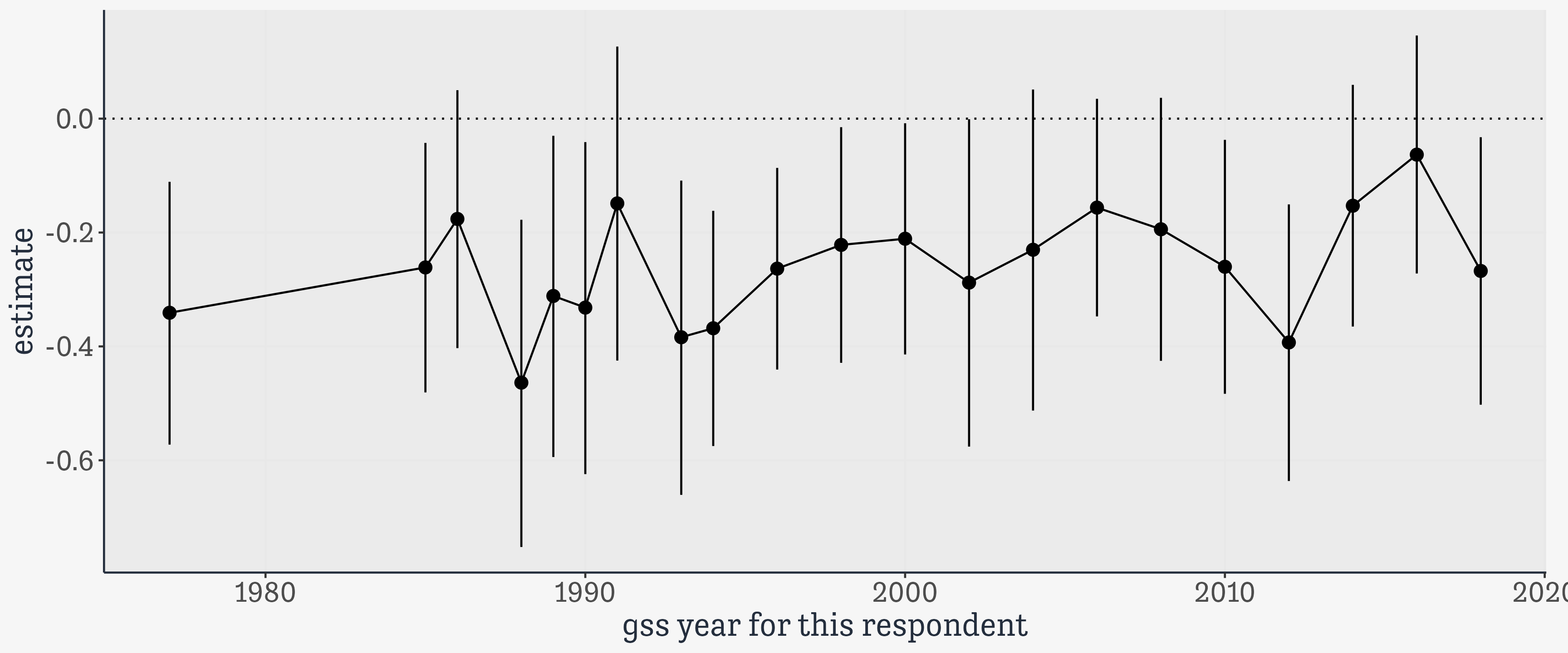
group_modify() and possibly()

out_yr |>
  filter(term == "sexFemale") |>
  ggplot(mapping = aes(x = year, y = estimate,
                       ymin = conf.low, ymax = conf.high)) +
  geom_hline(yintercept = 0, linetype = "dotted") +
  geom_line() +
  geom_pointrange()

Survey-weighted estimates

Those were still unweighted estimates. Weights are more complex.

options(survey.lonely.psu = "adjust")
options(na.action="na.pass")

gss_svy <- gss_df |>
  filter(year > 1974) |>
  mutate(stratvar = interaction(year, vstrat)) |>
  as_survey_design(id = vpsu,
                     strata = stratvar,
                     weights = wtssall,
                     nest = TRUE)
gss_svy

Stratified 1 - level Cluster Sampling design (with replacement)
With (4555) clusters.
Called via srvyr
Sampling variables:
  - ids: vpsu 
  - strata: stratvar 
  - weights: wtssall 
Data variables: 
  - year (dbl+lbl), id (dbl), ballot (dbl+lbl), age (dbl+lbl), race (fct), sex
    (fct), fefam (fct), vpsu (dbl), vstrat (dbl), oversamp (dbl), formwt (dbl),
    wtssall (dbl), sampcode (dbl), sample (dbl), compwt (dbl), fefam_d (fct),
    fefam_n (dbl), stratvar (fct)

Survey-weighted estimates

gss_svy |>
  drop_na(fefam_d) |>
  group_by(year, sex, race, fefam_d) |>
  summarize(prop = survey_mean(na.rm = TRUE,
                               vartype = "ci"))

# A tibble: 252 × 7
# Groups:   year, sex, race [126]
   year      sex    race  fefam_d   prop prop_low prop_upp
   <dbl+lbl> <fct>  <fct> <fct>    <dbl>    <dbl>    <dbl>
 1 1977      Male   White Agree    0.694   0.655     0.732
 2 1977      Male   White Disagree 0.306   0.268     0.345
 3 1977      Male   Black Agree    0.686   0.564     0.807
 4 1977      Male   Black Disagree 0.314   0.193     0.436
 5 1977      Male   Other Agree    0.632   0.357     0.906
 6 1977      Male   Other Disagree 0.368   0.0936    0.643
 7 1977      Female White Agree    0.640   0.601     0.680
 8 1977      Female White Disagree 0.360   0.320     0.399
 9 1977      Female Black Agree    0.553   0.472     0.634
10 1977      Female Black Disagree 0.447   0.366     0.528
# ℹ 242 more rows

Survey-weighted estimates

The entire dataset again.

out_svy_all <- svyglm(fefam_n ~ age + sex + race,
                  design = gss_svy,
                  family = quasibinomial(),
                  na.action = na.omit)

tidy(out_svy_all)

# A tibble: 5 × 5
  term        estimate std.error statistic   p.value
  <chr>          <dbl>     <dbl>     <dbl>     <dbl>
1 (Intercept)  -1.83    0.0478     -38.3   6.34e-234
2 age           0.0310  0.000852    36.4   9.99e-217
3 sexFemale    -0.235   0.0277      -8.48  4.55e- 17
4 raceBlack     0.0282  0.0432       0.653 5.14e-  1
5 raceOther     0.382   0.0588       6.50  1.06e- 10

And possibly() again

We should able to write this:

safe_svy_glm <- possibly(svyglm, otherwise = NULL)

tidy_svy_glm <- function(...){
  tidy(safe_svy_glm(...))
}

And use it with group_modify(), just the same as before. But we can’t. Alas, group_modify() isn’t (yet) implemented for srvyr objects. We have to use an older way of expressing the same idea.

Survey-weighted estimates, by year

We have to use group_map_dfr() and formula (~) notation in the possibly() call. Note the .x there, which is how the data frame gets passed in. (This way of writing things used to be more common.) We also can’t easily wrap the functions. So the result is more awkward:

out_svy_yrs <- gss_svy |>
  group_by(year) |>
  group_map_dfr(
    possibly(~ tidy(
      svyglm(fefam_n ~ age + sex + race, design = .x,
                       family = quasibinomial(),
                       na.action = na.omit),
                       conf.int = TRUE),
      otherwise = NULL
      )
  )

Survey-weighted estimates, by year

out_svy_yrs

# A tibble: 105 × 8
   year      term       estimate std.error statistic  p.value conf.low conf.high
   <dbl+lbl> <chr>         <dbl>     <dbl>     <dbl>    <dbl>    <dbl>     <dbl>
 1 1977      (Intercep…  -1.09     0.184      -5.93  3.74e- 7  -1.46    -0.720  
 2 1977      age          0.0469   0.00403    11.6   2.63e-15   0.0388   0.0550 
 3 1977      sexFemale   -0.344    0.126      -2.73  9.05e- 3  -0.599   -0.0901 
 4 1977      raceBlack   -0.144    0.215      -0.669 5.07e- 1  -0.576    0.288  
 5 1977      raceOther    0.276    0.552       0.500 6.19e- 1  -0.835    1.39   
 6 1985      (Intercep…  -1.89     0.199      -9.49  9.05e-13  -2.29    -1.49   
 7 1985      age          0.0431   0.00369    11.7   6.47e-16   0.0357   0.0505 
 8 1985      sexFemale   -0.174    0.123      -1.42  1.61e- 1  -0.421    0.0720 
 9 1985      raceBlack    0.157    0.228       0.688 4.95e- 1  -0.301    0.614  
10 1985      raceOther   -0.533    0.268      -1.99  5.24e- 2  -1.07     0.00573
# ℹ 95 more rows

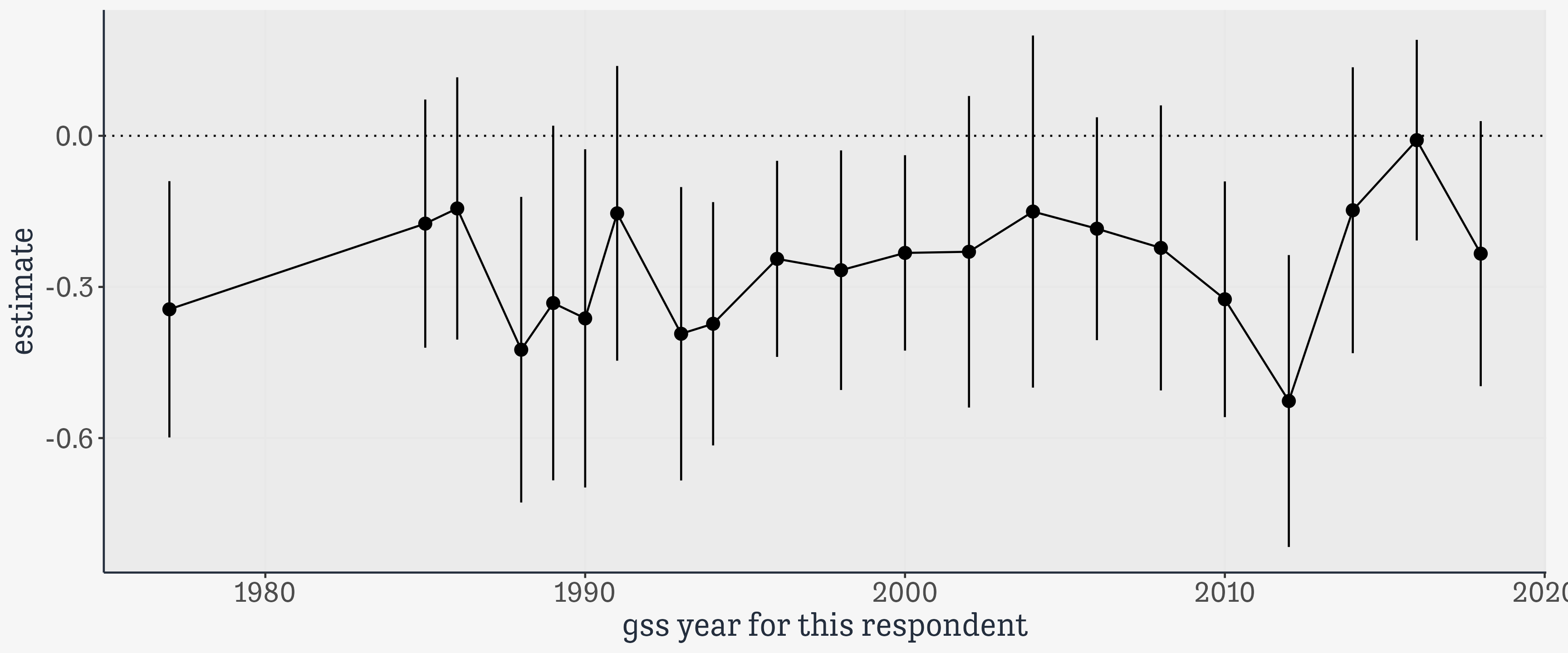
Survey-weighted estimates, by year

out_svy_yrs |>
  filter(term == "sexFemale") |>
  ggplot(mapping = aes(x = year,
                       y = estimate,
                       ymin = conf.low,
                       ymax = conf.high)) +
  geom_hline(yintercept = 0, linetype = "dotted") +
  geom_line() +
  geom_pointrange()