── Conflicts ────────────────────────────────────────── tidyverse_conflicts() ──
✖ dplyr::filter() masks stats::filter()
✖ dplyr::lag()    masks stats::lag()
ℹ Use the conflicted package (<http://conflicted.r-lib.org/>) to force all conflicts to become errors
Split
Apply
Combine
The Core Idea
Split or group the data into pieces
Apply a function, i.e. act on the data
Combine the results back into a table
Sometimes we start out in a “split” state, as when we have multiple data files, and we need to read them in and then combine them.
More than one data file
Inside files/examples/ is a folder named congress/
# A little trick from the fs package:fs::dir_tree(here("files", "examples", "congress"))
# A tibble: 6 × 25
  last     first   middle suffix nickname born  death sex   position party state
  <chr>    <chr>   <chr>  <chr>  <chr>    <chr> <chr> <chr> <chr>    <chr> <chr>
1 Abdnor   James   <NA>   <NA>   <NA>     02/1… 11/0… M     U.S. Re… Repu… SD
2 Abourezk James   George <NA>   <NA>     02/2… <NA>  M     U.S. Se… Demo… SD
3 Adams    Brockm… <NA>   <NA>   Brock    01/1… 09/1… M     U.S. Re… Demo… WA
4 Addabbo  Joseph  Patri… <NA>   <NA>     03/1… 04/1… M     U.S. Re… Demo… NY
5 Aiken    George  David  <NA>   <NA>     08/2… 11/1… M     U.S. Se… Repu… VT
6 Akaka    Daniel  Kahik… <NA>   <NA>     09/1… 04/0… M     U.S. Re… Demo… HI
# ℹ 14 more variables: district <chr>, start <chr>, end <chr>, religion <chr>,
#   race <chr>, educational_attainment <chr>, job_type1 <chr>, job_type2 <chr>,
#   job_type3 <chr>, job_type4 <chr>, job_type5 <lgl>, mil1 <chr>, mil2 <chr>,
#   mil3 <chr>
We often find ourselves in this situation. We know each file has the same structure, and we would like to use them all at once.
Loops?
How to read them all in?
One traditional way, which we could do in R, is to write an explicit loop that iterated over a vector of filenames, read each file, and then stack the results all together in a tall rectangle.
## Pseudocode (i.e. will not really run)## Also, if you do write loops, do not use them to grow dataframes in this way.filenames <-c("01_79_congress.csv", "02_80_congress.csv", "03_81_congress.csv","04_82_congress.csv" [etc etc])collected_files <-NULLfor(i in1:length(filenames)) { new_file <-read_file(filenames[i]) collected_files <-append_to(collected_files, new_files)}
A for loop initializes a counter and goes around and around, doing the thing and incrementing the counter until reaching a defined max value. A while loop keeps going until some condition is met.
Loops?
You may have noticed we have not written any loops, however.
While loops are still lurking there underneath the surface, what we will do instead is to take advantage of the combination of functions and vectors (or tables) and apply or map one to the other in order to generate results.
Speaking loosely, think of map() as a way of iterating without explicitly writing loops. You start with a vector of things. You feed it one thing at a time to some function. The function does whatever it does. You get back output that is the same length as your input, and of a specific type.
The reason we do this is that it leads to code we can pipeline as a sequence of function calls.
Mapping is just a kind of iteration
The purrr package provides a big family of mapping functions. One reason there are a lot of them is that purrr, like the rest of the tidyverse, is picky about data types.
So in addition to the basic map(), which always returns a list, we also have map_chr(), map_int(), map_dbl(), map_lgl() and others.
There are also variants for mapping over multiple inputs at once, like map2(), for when we are passing two arugments to some function, and pmap(), when we want to pass a list of any number of arguments.
The first part of the name tells you how many arguments are passing (1, 2, many). The part after the underscore tells you what type of output to expect. If there’s no suffix, you get a list back. These functions return their promised type or die trying.
Vectorized arithmetic again
The simplest cases are not that different from the vectorized arithmetic we’re already familiar with.
a <-c(1:10)b <-1# You know what R will do herea + b
[1] 2 3 4 5 6 7 8 9 10 11
R’s vectorized rules add b to every element of a. The + operation can be thought of as a function that takes each element of a and does something with it. In this case “add b”. This is already a kind of iteration, in the sense that the operation recycles b down the vector a (unless they are the same length).
Vectorized arithmetic again
We can make this explicit by writing a function:
add_b <-function(x) { b <-1# fixed x + b # for any valid x}
Vectorized arithmetic again
We can make this explicit by writing a function:
add_b <-function(x) { b <-1 x + b # for any x}
Now:
add_b(x = a)
[1] 2 3 4 5 6 7 8 9 10 11
Vectorized arithmetic again
Again, R’s vectorized approach means it automatically adds b to every element of the x we give it.
add_b(x =10)
[1] 11
add_b(x =c(1, 99, 1000))
[1] 2 100 1001
Iterating in a pipeline
Some operations can’t directly be vectorized in this way, which is why we need to manually iterate, which will make us want to write loops.
library(gapminder)# Not what we want in this casegapminder |>n_distinct()
[1] 1704
When you find yourself saying “No, I meant for each …”
That’s tedious to write! Computers are meant to let us avoid this sort of thing.
Iterating in a pipeline
So how would we iterate this? What we want is to apply the n_distinct() function to each column of gapminder, but in a way that still allows us to use pipelines and so on. Here we leave out the names so we can see that the result is literally the same function being applied to each column.
# A tibble: 1 × 6
  country continent  year lifeExp   pop gdpPercap
    <int>     <int> <int>   <int> <int>     <int>
1     142         5    12    1626  1704      1704
In this context, the function is applied across the specified columns; you’re always getting a tibble back; and the names are taken care of automatically.
result <- gapminder |>map(n_distinct)class(result)
[1] "list"
result$continent
[1] 5
result[[2]]
[1] 5
Iterating in a pipeline
But we know n_distinct() should always return an integer. We just want a vector of integers back, not a list of them. So we use map_int() instead of the generic map().
gapminder |>map_int(n_distinct)
  country continent      year   lifeExp       pop gdpPercap
      142         5        12      1626      1704      1704
The map() family can deal with all kinds of input types and output types. We choose some specific variant of map based on two things: what (and how many) things we are feeding the function we’re mapping, and what type of thing it should return.
Get a vector of filenames
filenames <-dir(path =here("files", "examples", "congress"),pattern ="*.csv",full.names =TRUE)filenames[1:15] # Just displaying the first 15, to save slide space
# A tibble: 20,580 × 26
   congress last   first middle suffix nickname born  death sex   position party
      <int> <chr>  <chr> <chr>  <chr>  <chr>    <chr> <chr> <chr> <chr>    <chr>
 1        1 Abern… Thom… Gerst… <NA>   <NA>     05/1… 01/2… M     U.S. Re… Demo…
 2        1 Adams  Sher… <NA>   <NA>   <NA>     01/0… 10/2… M     U.S. Re… Repu…
 3        1 Aiken  Geor… David  <NA>   <NA>     08/2… 11/1… M     U.S. Se… Repu…
 4        1 Allen  Asa   Leona… <NA>   <NA>     01/0… 01/0… M     U.S. Re… Demo…
 5        1 Allen  Leo   Elwood <NA>   <NA>     10/0… 01/1… M     U.S. Re… Repu…
 6        1 Almond J.    Linds… Jr.    <NA>     06/1… 04/1… M     U.S. Re… Demo…
 7        1 Ander… Herm… Carl   <NA>   <NA>     01/2… 07/2… M     U.S. Re… Repu…
 8        1 Ander… Clin… Presba <NA>   <NA>     10/2… 11/1… M     U.S. Re… Demo…
 9        1 Ander… John  Zuing… <NA>   <NA>     03/2… 02/0… M     U.S. Re… Repu…
10        1 Andre… Augu… Herman <NA>   <NA>     10/1… 01/1… M     U.S. Re… Repu…
# ℹ 20,570 more rows
# ℹ 15 more variables: state <chr>, district <chr>, start <chr>, end <chr>,
#   religion <chr>, race <chr>, educational_attainment <chr>, job_type1 <chr>,
#   job_type2 <chr>, job_type3 <chr>, job_type4 <chr>, job_type5 <chr>,
#   mil1 <chr>, mil2 <chr>, mil3 <chr>
read_csv() can do this directly
In fact map() is not required for this particular use:
# A tibble: 20,580 × 27
   congress path   last  first middle suffix nickname born  death sex   position
   <chr>    <chr>  <chr> <chr> <chr>  <chr>  <chr>    <chr> <chr> <chr> <chr>
 1 79       /User… Aber… Thom… Gerst… <NA>   <NA>     05/1… 01/2… M     U.S. Re…
 2 79       /User… Adams Sher… <NA>   <NA>   <NA>     01/0… 10/2… M     U.S. Re…
 3 79       /User… Aiken Geor… David  <NA>   <NA>     08/2… 11/1… M     U.S. Se…
 4 79       /User… Allen Asa   Leona… <NA>   <NA>     01/0… 01/0… M     U.S. Re…
 5 79       /User… Allen Leo   Elwood <NA>   <NA>     10/0… 01/1… M     U.S. Re…
 6 79       /User… Almo… J.    Linds… Jr.    <NA>     06/1… 04/1… M     U.S. Re…
 7 79       /User… Ande… Herm… Carl   <NA>   <NA>     01/2… 07/2… M     U.S. Re…
 8 79       /User… Ande… Clin… Presba <NA>   <NA>     10/2… 11/1… M     U.S. Re…
 9 79       /User… Ande… John  Zuing… <NA>   <NA>     03/2… 02/0… M     U.S. Re…
10 79       /User… Andr… Augu… Herman <NA>   <NA>     10/1… 01/1… M     U.S. Re…
# ℹ 20,570 more rows
# ℹ 16 more variables: party <chr>, state <chr>, district <chr>, start <chr>,
#   end <chr>, religion <chr>, race <chr>, educational_attainment <chr>,
#   job_type1 <chr>, job_type2 <chr>, job_type3 <chr>, job_type4 <chr>,
#   job_type5 <chr>, mil1 <chr>, mil2 <chr>, mil3 <chr>
Wrangling Models
This is not a statistics seminar!
I’ll just give you an example of the sort of thing that many other modeling packages implement for all kinds of modeling techniques.
Again, the principle is tidy incorporation of models and their output.
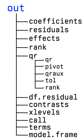
Which means, as always: tibbles. We want a data frame of our results. A nice rectangular table that we know what to do with regardless of what its contents mean.
That’s a lot nicer. Now it’s just a tibble. We know those. This is only a small piece of what’s in the summary object, but we’ll get to the rest in a minute.
Residual standard error: 8.336 on 1697 degrees of freedom
Multiple R-squared:  0.585, Adjusted R-squared:  0.5835
F-statistic: 398.7 on 6 and 1697 DF,  p-value: < 2.2e-16
Residual standard error: 8.336 on 1697 degrees of freedom
Multiple R-squared:  0.585, Adjusted R-squared:  0.5835
F-statistic: 398.7 on 6 and 1697 DF,  p-value: < 2.2e-16
Residual standard error:8.336 on 1697 degrees of freedomMultiple R-squared:0.585, Adjusted R-squared:0.5835F-statistic:398.7 on 6 and 1697 DF, p-value:<2.2e-16
The usefulness of glance() becomes clearer when dealing with ensembles of models.
Grouped Analysis
Grouped analysis and list columns
European countries in 1977:
gapminder |>filter(continent =="Europe", year ==1977)
# A tibble: 30 × 6
   country                continent  year lifeExp      pop gdpPercap
   <fct>                  <fct>     <int>   <dbl>    <int>     <dbl>
 1 Albania                Europe     1977    68.9  2509048     3533.
 2 Austria                Europe     1977    72.2  7568430    19749.
 3 Belgium                Europe     1977    72.8  9821800    19118.
 4 Bosnia and Herzegovina Europe     1977    69.9  4086000     3528.
 5 Bulgaria               Europe     1977    70.8  8797022     7612.
 6 Croatia                Europe     1977    70.6  4318673    11305.
 7 Czech Republic         Europe     1977    70.7 10161915    14800.
 8 Denmark                Europe     1977    74.7  5088419    20423.
 9 Finland                Europe     1977    72.5  4738902    15605.
10 France                 Europe     1977    73.8 53165019    18293.
# ℹ 20 more rows
Let’s fit a simple model predicting life expectancy from GDP per capita for just these countries.
Grouped analysis and list columns
eu77 <- gapminder |>filter(continent =="Europe", year ==1977)fit <-lm(lifeExp ~log(gdpPercap), data = eu77)
summary(fit)
Call:
lm(formula = lifeExp ~ log(gdpPercap), data = eu77)

Residuals:
    Min      1Q  Median      3Q     Max
-7.4956 -1.0306  0.0935  1.1755  3.7125

Coefficients:
               Estimate Std. Error t value Pr(>|t|)
(Intercept)      29.489      7.161   4.118 0.000306 ***
log(gdpPercap)    4.488      0.756   5.936 2.17e-06 ***
---
Signif. codes:  0 '***' 0.001 '**' 0.01 '*' 0.05 '.' 0.1 ' ' 1

Residual standard error: 2.114 on 28 degrees of freedom
Multiple R-squared:  0.5572,    Adjusted R-squared:  0.5414
F-statistic: 35.24 on 1 and 28 DF,  p-value: 2.173e-06
What if we want to do this for every continent in every year?
# A tibble: 60 × 3
# Groups:   continent, year [60]
   continent  year data
   <fct>     <int> <list>
 1 Asia       1952 <tibble [33 × 4]>
 2 Asia       1957 <tibble [33 × 4]>
 3 Asia       1962 <tibble [33 × 4]>
 4 Asia       1967 <tibble [33 × 4]>
 5 Asia       1972 <tibble [33 × 4]>
 6 Asia       1977 <tibble [33 × 4]>
 7 Asia       1982 <tibble [33 × 4]>
 8 Asia       1987 <tibble [33 × 4]>
 9 Asia       1992 <tibble [33 × 4]>
10 Asia       1997 <tibble [33 × 4]>
# ℹ 50 more rows
Think of nesting as a kind of “super-grouping”. Look in the object inspector.
Grouped analysis and list columns
It’s still in there.
df_nest|>filter(continent =="Europe"& year ==1977) |>unnest(cols =c(data))
# A tibble: 30 × 6
# Groups:   continent, year [1]
   continent  year country                lifeExp      pop gdpPercap
   <fct>     <int> <fct>                    <dbl>    <int>     <dbl>
 1 Europe     1977 Albania                   68.9  2509048     3533.
 2 Europe     1977 Austria                   72.2  7568430    19749.
 3 Europe     1977 Belgium                   72.8  9821800    19118.
 4 Europe     1977 Bosnia and Herzegovina    69.9  4086000     3528.
 5 Europe     1977 Bulgaria                  70.8  8797022     7612.
 6 Europe     1977 Croatia                   70.6  4318673    11305.
 7 Europe     1977 Czech Republic            70.7 10161915    14800.
 8 Europe     1977 Denmark                   74.7  5088419    20423.
 9 Europe     1977 Finland                   72.5  4738902    15605.
10 Europe     1977 France                    73.8 53165019    18293.
# ℹ 20 more rows
Grouped analysis and list columns
Here we map() a custom function to every row in the data column.
## Keep everything, do the matching and weighting inside the bootboot_out <-tibble(boot_id =1:n_replicates) |>mutate(boot_data =map(boot_id, \(x) slice_sample(lalonde, n =nrow(lalonde),replace =TRUE)),match_obj =map(boot_data, \(bd) { matchit(treat ~ age + educ + race + married + nodegree + re74 + re75,data = bd,method ="nearest",estimand ="ATT") }),model =map2(boot_data, match_obj, \(bd, mo) { lm(re78 ~ treat + age + educ + race + married + nodegree + re74 + re75,data = bd,weights = mo$weights) }),coefs =map(model, tidy) )
Four map() calls including one to map2(). We could separately write named functions for the steps inside the mapping calls, but we use lambdas instead and write them on the fly.
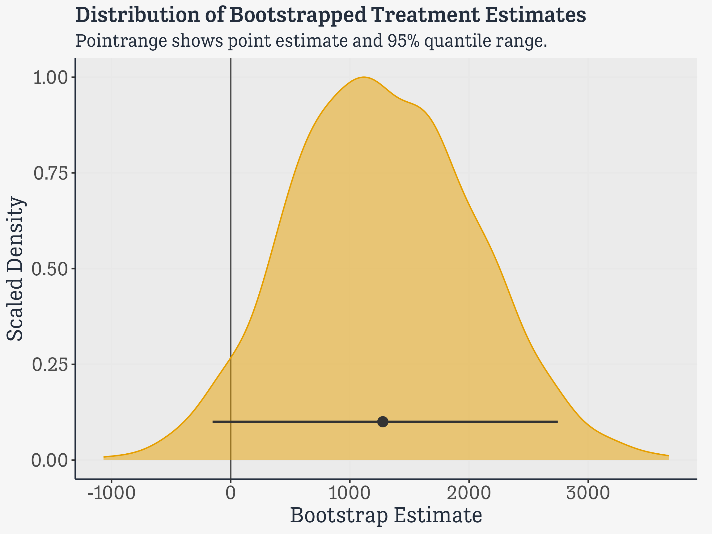
# Simplest way to calculate bootstrap ci's; could get# much fancier using boot() or any number of other fns for the# bootstrap stageboot_tbl <- boot_out |>unnest(coefs) |>filter(term =="treat") |>summarize(boot_att =mean(estimate),boot_se =sd(estimate),boot_ci_lower =quantile(estimate, 0.025),boot_ci_upper =quantile(estimate, 0.975) )tinytable::tt(boot_tbl, digits =3)
boot_att
boot_se
boot_ci_lower
boot_ci_upper
1276
761
-152
2744
Bootstrapped ATT estimates
tmp_tbl <- boot_tbl |>mutate(y =0.1)boot_out |>unnest(coefs) |>select(boot_id, term, estimate) |>filter(term =="treat") |>ggplot(mapping =aes(x = estimate, y =after_stat(scaled),color = term, fill = term)) +geom_vline(xintercept =0, color ="gray30") +geom_density(alpha =0.5) +geom_pointrange(data = tmp_tbl,mapping =aes(x = boot_att, y = y, xmin = boot_ci_lower,xmax = boot_ci_upper),color ="gray20", size =rel(0.7), linewidth =rel(0.9),inherit.aes =FALSE) +labs(title ="Distribution of Bootstrapped Treatment Estimates",subtitle ="Pointrange shows point estimate and 95% quantile range.",x ="Bootstrap Estimate", y ="Scaled Density") +guides(color ="none", fill ="none")
Bootstrapped ATT estimates
Distribution of Treatment Estimates
Midwest PCA Example
Midwest data
midwest
# A tibble: 437 × 28
     PID county  state  area poptotal popdensity popwhite popblack popamerindian
   <int> <chr>   <chr> <dbl>    <int>      <dbl>    <int>    <int>         <int>
 1   561 ADAMS   IL    0.052    66090      1271.    63917     1702            98
 2   562 ALEXAN… IL    0.014    10626       759      7054     3496            19
 3   563 BOND    IL    0.022    14991       681.    14477      429            35
 4   564 BOONE   IL    0.017    30806      1812.    29344      127            46
 5   565 BROWN   IL    0.018     5836       324.     5264      547            14
 6   566 BUREAU  IL    0.05     35688       714.    35157       50            65
 7   567 CALHOUN IL    0.017     5322       313.     5298        1             8
 8   568 CARROLL IL    0.027    16805       622.    16519      111            30
 9   569 CASS    IL    0.024    13437       560.    13384       16             8
10   570 CHAMPA… IL    0.058   173025      2983.   146506    16559           331
# ℹ 427 more rows
# ℹ 19 more variables: popasian <int>, popother <int>, percwhite <dbl>,
#   percblack <dbl>, percamerindan <dbl>, percasian <dbl>, percother <dbl>,
#   popadults <int>, perchsd <dbl>, percollege <dbl>, percprof <dbl>,
#   poppovertyknown <int>, percpovertyknown <dbl>, percbelowpoverty <dbl>,
#   percchildbelowpovert <dbl>, percadultpoverty <dbl>,
#   percelderlypoverty <dbl>, inmetro <int>, category <chr>
# A tibble: 5 × 3
# Groups:   state [5]
  state data                pca
  <chr> <list>              <list>
1 IL    <tibble [102 × 24]> <prcomp>
2 IN    <tibble [92 × 24]>  <prcomp>
3 MI    <tibble [83 × 24]>  <prcomp>
4 OH    <tibble [88 × 24]>  <prcomp>
5 WI    <tibble [72 × 24]>  <prcomp>
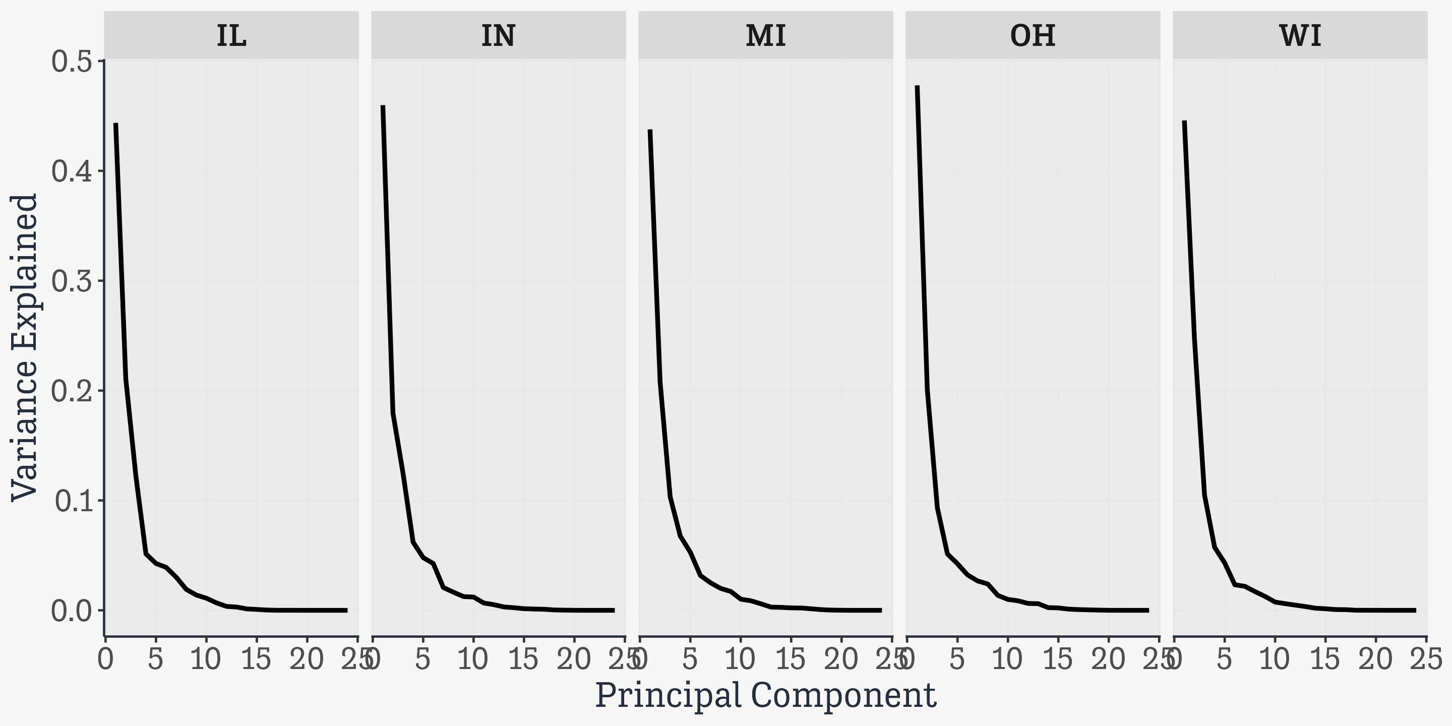
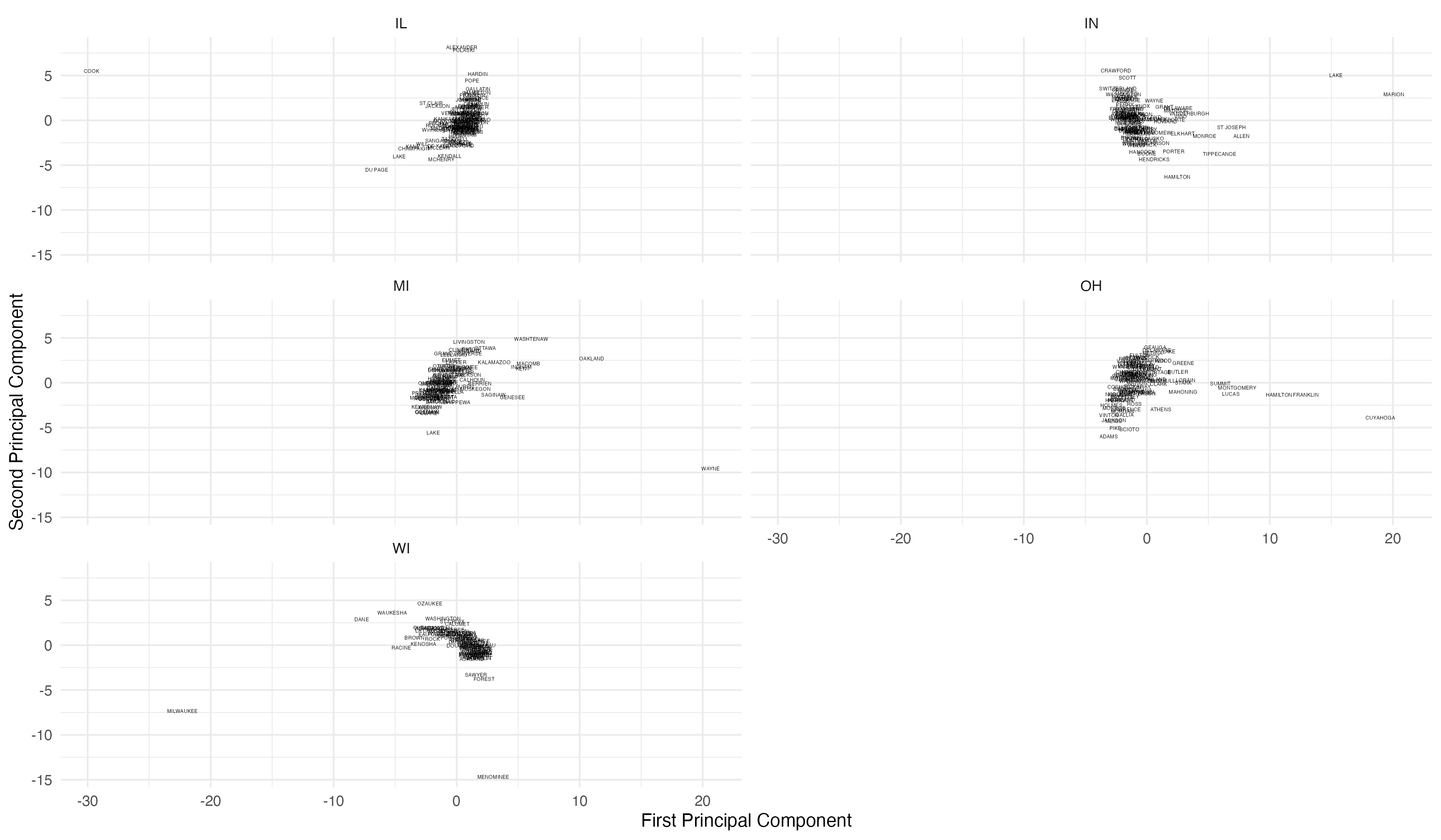
Grouped PCA
Alternatively, write a lambda function:
mw_pca |>mutate(pca =map(data, \(x) prcomp(x, center =TRUE, scale =TRUE)))
# A tibble: 5 × 3
# Groups:   state [5]
  state data                pca
  <chr> <list>              <list>
1 IL    <tibble [102 × 24]> <prcomp>
2 IN    <tibble [92 × 24]>  <prcomp>
3 MI    <tibble [83 × 24]>  <prcomp>
4 OH    <tibble [88 × 24]>  <prcomp>
5 WI    <tibble [72 × 24]>  <prcomp>
Tidy it
# broom has methods for different models, including prcomp, and they take# arguments specific to those models. Here we want the principal components.do_tidy <-function(pr){ broom::tidy(pr, matrix ="pcs")}state_pca <- mw_pca |>mutate(pca =map(data, do_pca),pcs =map(pca, do_tidy))state_pca
# A tibble: 5 × 4
# Groups:   state [5]
  state data                pca      pcs
  <chr> <list>              <list>   <list>
1 IL    <tibble [102 × 24]> <prcomp> <tibble [24 × 4]>
2 IN    <tibble [92 × 24]>  <prcomp> <tibble [24 × 4]>
3 MI    <tibble [83 × 24]>  <prcomp> <tibble [24 × 4]>
4 OH    <tibble [88 × 24]>  <prcomp> <tibble [24 × 4]>
5 WI    <tibble [72 × 24]>  <prcomp> <tibble [24 × 4]>

 Crossover Event