Parallel Computing

Modern Plain Text Social Science
Week 11

Kieran Healy

Duke University

November 2025

Load the packages, as always

library(here)      # manage file paths
library(socviz)    # data and some useful functions
library(tidyverse) # your friend and mine

Split

Apply

Combine

For example

As you know by now, dplyr is all about this.

gss_sm |>
  count(bigregion)

# A tibble: 4 × 2
  bigregion     n
  <fct>     <int>
1 Northeast   488
2 Midwest     695
3 South      1052
4 West        632

We split into groups, apply the sum() function within the groups, and combine the results into a new tibble showing the resulting sum per group. The various dplyr functions are oriented to doing this in a way that gives you a consistent set of outputs.

For example: split

We can split, apply, combine in various ways.

Base R has the split() function:

out <- mtcars |>
  split(mtcars$cyl)
summary(out) # mtcars split into a list of data frames by the `cyl` variable

  Length Class      Mode
4 11     data.frame list
6 11     data.frame list
8 11     data.frame list

For example: split

Tidyverse has group_split():

out <- mtcars |>
  group_split(cyl)
out

<list_of<
  tbl_df<
    mpg : double
    cyl : double
    disp: double
    hp  : double
    drat: double
    wt  : double
    qsec: double
    vs  : double
    am  : double
    gear: double
    carb: double
  >
>[3]>
[[1]]
# A tibble: 11 × 11
     mpg   cyl  disp    hp  drat    wt  qsec    vs    am  gear  carb
   <dbl> <dbl> <dbl> <dbl> <dbl> <dbl> <dbl> <dbl> <dbl> <dbl> <dbl>
 1  22.8     4 108      93  3.85  2.32  18.6     1     1     4     1
 2  24.4     4 147.     62  3.69  3.19  20       1     0     4     2
 3  22.8     4 141.     95  3.92  3.15  22.9     1     0     4     2
 4  32.4     4  78.7    66  4.08  2.2   19.5     1     1     4     1
 5  30.4     4  75.7    52  4.93  1.62  18.5     1     1     4     2
 6  33.9     4  71.1    65  4.22  1.84  19.9     1     1     4     1
 7  21.5     4 120.     97  3.7   2.46  20.0     1     0     3     1
 8  27.3     4  79      66  4.08  1.94  18.9     1     1     4     1
 9  26       4 120.     91  4.43  2.14  16.7     0     1     5     2
10  30.4     4  95.1   113  3.77  1.51  16.9     1     1     5     2
11  21.4     4 121     109  4.11  2.78  18.6     1     1     4     2

[[2]]
# A tibble: 7 × 11
    mpg   cyl  disp    hp  drat    wt  qsec    vs    am  gear  carb
  <dbl> <dbl> <dbl> <dbl> <dbl> <dbl> <dbl> <dbl> <dbl> <dbl> <dbl>
1  21       6  160    110  3.9   2.62  16.5     0     1     4     4
2  21       6  160    110  3.9   2.88  17.0     0     1     4     4
3  21.4     6  258    110  3.08  3.22  19.4     1     0     3     1
4  18.1     6  225    105  2.76  3.46  20.2     1     0     3     1
5  19.2     6  168.   123  3.92  3.44  18.3     1     0     4     4
6  17.8     6  168.   123  3.92  3.44  18.9     1     0     4     4
7  19.7     6  145    175  3.62  2.77  15.5     0     1     5     6

[[3]]
# A tibble: 14 × 11
     mpg   cyl  disp    hp  drat    wt  qsec    vs    am  gear  carb
   <dbl> <dbl> <dbl> <dbl> <dbl> <dbl> <dbl> <dbl> <dbl> <dbl> <dbl>
 1  18.7     8  360    175  3.15  3.44  17.0     0     0     3     2
 2  14.3     8  360    245  3.21  3.57  15.8     0     0     3     4
 3  16.4     8  276.   180  3.07  4.07  17.4     0     0     3     3
 4  17.3     8  276.   180  3.07  3.73  17.6     0     0     3     3
 5  15.2     8  276.   180  3.07  3.78  18       0     0     3     3
 6  10.4     8  472    205  2.93  5.25  18.0     0     0     3     4
 7  10.4     8  460    215  3     5.42  17.8     0     0     3     4
 8  14.7     8  440    230  3.23  5.34  17.4     0     0     3     4
 9  15.5     8  318    150  2.76  3.52  16.9     0     0     3     2
10  15.2     8  304    150  3.15  3.44  17.3     0     0     3     2
11  13.3     8  350    245  3.73  3.84  15.4     0     0     3     4
12  19.2     8  400    175  3.08  3.84  17.0     0     0     3     2
13  15.8     8  351    264  4.22  3.17  14.5     0     1     5     4
14  15       8  301    335  3.54  3.57  14.6     0     1     5     8

For example: apply

The application step is “I want to fit a linear model to each piece”. We did this with nest() last time.

out <- mtcars |>
  group_split(cyl) |>
  map(\(df) lm(mpg ~ wt + hp + gear, data = df))

For example: apply

The application step is “I want to fit a linear model to each piece” and get a summary. Again, we did this with group_by() and nest() last time.

mtcars |>
  group_split(cyl) |>
  map(\(df) lm(mpg ~ wt + hp + gear, data = df))  |>
  map(summary) |>
  map_dbl("r.squared")

[1] 0.7301860 0.6597413 0.4995237

For example: combine

In this case the “combine” step is implicitly at the end: we get a vector of R squareds back, and it’s as long as the number of groups.

mtcars |>
  group_split(cyl) |>
  map(\(df) lm(mpg ~ wt + hp + gear, data = df))  |>
  map(summary) |>
  map_dbl("r.squared")

[1] 0.7301860 0.6597413 0.4995237

For example: apply

This is also what we’re doing more elegantly (staying within a tibble structure) if we nest() and use broom to get a summary out.

mtcars |>
  group_by(cyl) |>
  nest() |>
  mutate(model = map(data, \(df) lm(mpg ~ wt + hp + gear, data = df)),
         perf = map(model, broom::glance)) |>
  unnest(perf)

# A tibble: 3 × 15
# Groups:   cyl [3]
    cyl data     model  r.squared adj.r.squared sigma statistic p.value    df
  <dbl> <list>   <list>     <dbl>         <dbl> <dbl>     <dbl>   <dbl> <dbl>
1     6 <tibble> <lm>       0.660         0.319  1.20      1.94  0.300      3
2     4 <tibble> <lm>       0.730         0.615  2.80      6.31  0.0211     3
3     8 <tibble> <lm>       0.500         0.349  2.06      3.33  0.0648     3
# ℹ 6 more variables: logLik <dbl>, AIC <dbl>, BIC <dbl>, deviance <dbl>,
#   df.residual <int>, nobs <int>

How this happens

In each of these cases, the data is processed sequentially or serially. R splits the data according to your instructions, applies the function or procedure to each one in turn, and combines the outputs in order out the other side. Your computer’s processor is handed each piece in turn.

How this happens

For small tasks that’s fine. But for bigger tasks it gets inefficient quickly.

## From Henrik Bengtsson's documentation for future/furr
slow_sum <- function(x) {
  sum <- 0
  for (value in x) {
    Sys.sleep(1.0)  ## one-second slowdown per value
    sum <- sum + value
  }
  sum
}

# This takes > ten seconds to run.
tictoc::tic()
slow_sum(1:10)

[1] 55

tictoc::toc()

10.039 sec elapsed

If this is the sort of task we have to apply to a bunch of things, it’s going to take ages.

That’s Embarrassing

A feature of many split-apply-combine activities is that it does not matter what order the “apply” part happens to the groups. All that matters is that we can combine the results at the end, no matter what order they come back in. E.g. in the mtcars example the model being fit to the 4-cylinder cars group doesn’t depend in any way on the results of the model being fit to the 8-cylinder group.

This sort of situation is embarrassingly parallel.

That’s Embarrassing

When a task is embarrassingly parallel, and the number of pieces or groups is large enough or complex enough, then if we can do them at the same time then we should. There is some overhead—we have to keep track of where each piece was sent and when the results come back in—but if that’s low enough in comparison to doing things serially, then we should parallelize the task.

Multicore Computing

Parallel computing used to mean “I have a cluster of computers at my disposal”. But modern CPUs are constructed in a semi-modular fashion. They have some number of “cores”, each one of which is like a small processor in its own right. In effect you have a computer cluster already.

Some Terms

Socket: The physical connection on your computer that houses the processor. These days, mostly there’s just one.

Core: The part of the processor that actually performs the computation. Most modern processors have multiple cores. Each one can do wholly independent work.

Process: A single instance of a running task or program (R, Slack, Chrome, etc). A core can only run one process at a time. But, cores are fast. And so, they can run many threads

Some Terms

Thread: A piece of a process that can share memory and resources with other threads. If you have enough power you can do something Intel called hyperthreading, which is a way of dividing up a physical core into (usually) two logical cores that work on the same clock cycle and share some resources on the physical core.

Cluster: A collection of things that are capable of hosting cores. Might be a single socket (on your laptop) or an old-fashioned room full of many physical computers that can be made to act as if they were a single machine.

Multicore Computing

Most of the time, even when we are using them, our computers sit around doing PRETTY MUCH NOTHING.

## How many cores do we have?
parallel::detectCores()

[1] 16

Remember, processor clock cycles are really fast. They’re measured in billions of cycles per second. We need to put those cores to work!

Previously: Future and furrr

future and furrr made parallel computing way more straightforward than it used to be. In particular, for Tidyverse-centric workflows, furrr provides a set of future_ functions that are drop-in replacements for map and friends. So map() becomes future_map() and so on.

However, purrr has recently added support for parallelization via the in_parallel() function. It uses crate and mirai under the hood.

Parallel `purrr`

Update your R packages with remotes::update_packages().

library(tidyverse)
library(here)

# Set up parallel processing
library(mirai)

# Summon daemons. Do not summon more daemons than you have cores. People often choose one less than the number of cores.
daemons(15)
status()

$connections
[1] 15

$daemons
[1] "ipc:///tmp/74ae824ea49c3acf02834580"

$mirai
 awaiting executing completed 
        0         0         0

Toy Example

# Another slow function (from
# Grant McDermott this time)
slow_square <- function(x = 1) {
    x_sq <- x^2
    ## We explicitly namespace all our package function calls
    out <-  tibble::tibble(value = x, value_sq = x_sq)
    Sys.sleep(2) # Zzzz
    out
}

tictoc::tic("Serially")
## This is of course way slower than just writing
## slow_square(1:20) but nvm that for now
serial_out <- map(1:20, slow_square) |>
  list_rbind()
tictoc::toc()

Serially: 40.123 sec elapsed

Toy Example

tictoc::tic("Parallelized")
parallel_out <- 1:20 |>
  map(in_parallel(\(x) slow_square(x),
      slow_square = slow_square)) |>
        list_rbind()
tictoc::toc()

Parallelized: 4.172 sec elapsed

identical(serial_out, parallel_out)

[1] TRUE

Using `in_parallel()`

If you use in_parallel() but don’t set daemons(), then the map will just proceed sequentially, as if in_parallel() were not there.
You have to explicitly pass through the names of any local functions you’re using, as well as any local objects. This can make the code a little more verbose, but with more complex jobs it’s clear what’s being passed in and from where.
If you have written a local function and are passing that along, you must make sure any package functions it calls are fully namespaced (e.g. tibble::tibble() rather than just tibble()).

Using `in_parallel()`

E.g. From the help:

# ❌ This won't work - external dependencies not declared
my_data <- c(1, 2, 3)
map(1:3, in_parallel(\(x) mean(my_data)))

# ✅ This works - dependencies explicitly provided
my_data <- c(1, 2, 3)
map(1:3, in_parallel(\(x) mean(my_data), my_data = my_data))

# ✅ Package functions need explicit namespacing
map(1:3, in_parallel(\(x) vctrs::vec_init(integer(), x)))

# ✅ Or load packages within the function
map(
  1:3,
  in_parallel(\(x) {
    library(vctrs)
    vec_init(integer(), x)
  })

Extended Example

NOAA Temperature Data

See: https://github.com/kjhealy/noaa_ncei/. This function gets one folder full of NCDF files from NOAA.

#' Get a year-month folder of NCDF Files from NOAA
#'
#' @param url The endpoint URL of the AVHRR data, <https://www.ncei.noaa.gov/data/sea-surface-temperature-optimum-interpolation/v2.1/access/avhrr/>
#' @param local A local file path for the raw data folders, i.e. where all the year-month dirs go. Defaults to a local version under raw/ of the same path as the NOAA website.
#' @param subdir The subdirectory of monthly data to get. A character string of digits, of the form "YYYYMM". No default. Gets appended to `local`
#'
#' @return  A directory of NCDF files.
#' @export
#'
#'
get_nc_files <- function(
  url = "https://www.ncei.noaa.gov/data/sea-surface-temperature-optimum-interpolation/v2.1/access/avhrr/",
  local = here::here(
    "raw/www.ncei.noaa.gov/data/sea-surface-temperature-optimum-interpolation/v2.1/access/avhrr/"
  ),
  subdir
) {
  localdir <- here::here(local, subdir)

  if (!fs::dir_exists(localdir)) {
    fs::dir_create(localdir)
  }

  files <- rvest::read_html(paste0(url, subdir)) |>
    rvest::html_elements("a") |>
    rvest::html_text2()
  files <- subset(files, str_detect(files, "nc"))

  full_urls <- paste0(url, subdir, "/", files)
  full_outpaths <- paste0(localdir, "/", files)

  walk2(full_urls, full_outpaths, \(x, y) {
    httr::GET(x, httr::write_disk(y, overwrite = TRUE))
  })
}

NOAA Temperature Data

Initial get:

## Functions, incl. actual get_nc_files() function to get 1 year-month's batch of files.
source(here("R", "functions.R"))

### Initial get. Only have to do this once.
## We try to be nice.

# Data collection starts in September 1981
first_yr <- paste0("1981", sprintf('%0.2d', 9:12))
yrs <- 1982:2024
months <- sprintf('%0.2d', 1:12)
subdirs <- c(first_yr, paste0(rep(yrs, each = 12), months))

slowly_get_nc_files <- slowly(get_nc_files)

walk(subdirs, \(x) slowly_get_nc_files(subdir = x))

This tries to be polite with the NOAA: it enforces a wait time and in addition randomizes it to make it variably longer. There are a lot of files (>15,000). Doing it this way will take several days in real time (though much much less in actual transfer time of course).

NOAA Temperature Data

Raw data directories locally:

basename(fs::dir_ls(here::here("avhrr")))

  [1] "198109" "198110" "198111" "198112" "198201" "198202" "198203" "198204"
  [9] "198205" "198206" "198207" "198208" "198209" "198210" "198211" "198212"
 [17] "198301" "198302" "198303" "198304" "198305" "198306" "198307" "198308"
 [25] "198309" "198310" "198311" "198312" "198401" "198402" "198403" "198404"
 [33] "198405" "198406" "198407" "198408" "198409" "198410" "198411" "198412"
 [41] "198501" "198502" "198503" "198504" "198505" "198506" "198507" "198508"
 [49] "198509" "198510" "198511" "198512" "198601" "198602" "198603" "198604"
 [57] "198605" "198606" "198607" "198608" "198609" "198610" "198611" "198612"
 [65] "198701" "198702" "198703" "198704" "198705" "198706" "198707" "198708"
 [73] "198709" "198710" "198711" "198712" "198801" "198802" "198803" "198804"
 [81] "198805" "198806" "198807" "198808" "198809" "198810" "198811" "198812"
 [89] "198901" "198902" "198903" "198904" "198905" "198906" "198907" "198908"
 [97] "198909" "198910" "198911" "198912" "199001" "199002" "199003" "199004"
[105] "199005" "199006" "199007" "199008" "199009" "199010" "199011" "199012"
[113] "199101" "199102" "199103" "199104" "199105" "199106" "199107" "199108"
[121] "199109" "199110" "199111" "199112" "199201" "199202" "199203" "199204"
[129] "199205" "199206" "199207" "199208" "199209" "199210" "199211" "199212"
[137] "199301" "199302" "199303" "199304" "199305" "199306" "199307" "199308"
[145] "199309" "199310" "199311" "199312" "199401" "199402" "199403" "199404"
[153] "199405" "199406" "199407" "199408" "199409" "199410" "199411" "199412"
[161] "199501" "199502" "199503" "199504" "199505" "199506" "199507" "199508"
[169] "199509" "199510" "199511" "199512" "199601" "199602" "199603" "199604"
[177] "199605" "199606" "199607" "199608" "199609" "199610" "199611" "199612"
[185] "199701" "199702" "199703" "199704" "199705" "199706" "199707" "199708"
[193] "199709" "199710" "199711" "199712" "199801" "199802" "199803" "199804"
[201] "199805" "199806" "199807" "199808" "199809" "199810" "199811" "199812"
[209] "199901" "199902" "199903" "199904" "199905" "199906" "199907" "199908"
[217] "199909" "199910" "199911" "199912" "200001" "200002" "200003" "200004"
[225] "200005" "200006" "200007" "200008" "200009" "200010" "200011" "200012"
[233] "200101" "200102" "200103" "200104" "200105" "200106" "200107" "200108"
[241] "200109" "200110" "200111" "200112" "200201" "200202" "200203" "200204"
[249] "200205" "200206" "200207" "200208" "200209" "200210" "200211" "200212"
[257] "200301" "200302" "200303" "200304" "200305" "200306" "200307" "200308"
[265] "200309" "200310" "200311" "200312" "200401" "200402" "200403" "200404"
[273] "200405" "200406" "200407" "200408" "200409" "200410" "200411" "200412"
[281] "200501" "200502" "200503" "200504" "200505" "200506" "200507" "200508"
[289] "200509" "200510" "200511" "200512" "200601" "200602" "200603" "200604"
[297] "200605" "200606" "200607" "200608" "200609" "200610" "200611" "200612"
[305] "200701" "200702" "200703" "200704" "200705" "200706" "200707" "200708"
[313] "200709" "200710" "200711" "200712" "200801" "200802" "200803" "200804"
[321] "200805" "200806" "200807" "200808" "200809" "200810" "200811" "200812"
[329] "200901" "200902" "200903" "200904" "200905" "200906" "200907" "200908"
[337] "200909" "200910" "200911" "200912" "201001" "201002" "201003" "201004"
[345] "201005" "201006" "201007" "201008" "201009" "201010" "201011" "201012"
[353] "201101" "201102" "201103" "201104" "201105" "201106" "201107" "201108"
[361] "201109" "201110" "201111" "201112" "201201" "201202" "201203" "201204"
[369] "201205" "201206" "201207" "201208" "201209" "201210" "201211" "201212"
[377] "201301" "201302" "201303" "201304" "201305" "201306" "201307" "201308"
[385] "201309" "201310" "201311" "201312" "201401" "201402" "201403" "201404"
[393] "201405" "201406" "201407" "201408" "201409" "201410" "201411" "201412"
[401] "201501" "201502" "201503" "201504" "201505" "201506" "201507" "201508"
[409] "201509" "201510" "201511" "201512" "201601" "201602" "201603" "201604"
[417] "201605" "201606" "201607" "201608" "201609" "201610" "201611" "201612"
[425] "201701" "201702" "201703" "201704" "201705" "201706" "201707" "201708"
[433] "201709" "201710" "201711" "201712" "201801" "201802" "201803" "201804"
[441] "201805" "201806" "201807" "201808" "201809" "201810" "201811" "201812"
[449] "201901" "201902" "201903" "201904" "201905" "201906" "201907" "201908"
[457] "201909" "201910" "201911" "201912" "202001" "202002" "202003" "202004"
[465] "202005" "202006" "202007" "202008" "202009" "202010" "202011" "202012"
[473] "202101" "202102" "202103" "202104" "202105" "202106" "202107" "202108"
[481] "202109" "202110" "202111" "202112" "202201" "202202" "202203" "202204"
[489] "202205" "202206" "202207" "202208" "202209" "202210" "202211" "202212"
[497] "202301" "202302" "202303" "202304" "202305" "202306" "202307" "202308"
[505] "202309" "202310" "202311" "202312" "202401" "202402" "202403" "202404"
[513] "202405" "202406" "202407" "202408" "202409" "202410" "202411" "202412"
[521] "202501" "202502" "202503" "202504" "202505" "202506" "202507" "202508"

NOAA Temperature Data

Raw data files, in netCDF (Version 4) format

basename(fs::dir_ls(here::here("avhrr", "202402")))

 [1] "oisst-avhrr-v02r01.20240201.nc" "oisst-avhrr-v02r01.20240202.nc"
 [3] "oisst-avhrr-v02r01.20240203.nc" "oisst-avhrr-v02r01.20240204.nc"
 [5] "oisst-avhrr-v02r01.20240205.nc" "oisst-avhrr-v02r01.20240206.nc"
 [7] "oisst-avhrr-v02r01.20240207.nc" "oisst-avhrr-v02r01.20240208.nc"
 [9] "oisst-avhrr-v02r01.20240209.nc" "oisst-avhrr-v02r01.20240210.nc"
[11] "oisst-avhrr-v02r01.20240211.nc" "oisst-avhrr-v02r01.20240212.nc"
[13] "oisst-avhrr-v02r01.20240213.nc" "oisst-avhrr-v02r01.20240214.nc"
[15] "oisst-avhrr-v02r01.20240215.nc" "oisst-avhrr-v02r01.20240216.nc"
[17] "oisst-avhrr-v02r01.20240217.nc" "oisst-avhrr-v02r01.20240218.nc"
[19] "oisst-avhrr-v02r01.20240219.nc" "oisst-avhrr-v02r01.20240220.nc"
[21] "oisst-avhrr-v02r01.20240221.nc" "oisst-avhrr-v02r01.20240222.nc"
[23] "oisst-avhrr-v02r01.20240223.nc" "oisst-avhrr-v02r01.20240224.nc"
[25] "oisst-avhrr-v02r01.20240225.nc" "oisst-avhrr-v02r01.20240226.nc"
[27] "oisst-avhrr-v02r01.20240227.nc" "oisst-avhrr-v02r01.20240228.nc"
[29] "oisst-avhrr-v02r01.20240229.nc"

Some Prep

## Seasons for plotting
season <-  function(in_date){
  br = yday(as.Date(c("2019-03-01",
                      "2019-06-01",
                      "2019-09-01",
                      "2019-12-01")))
  x = yday(in_date)
  x = cut(x, breaks = c(0, br, 366))
  levels(x) = c("Winter", "Spring", "Summer", "Autumn", "Winter")
  x
}

season_lab <-  tibble(yrday = yday(as.Date(c("2019-03-01",
                                             "2019-06-01",
                                             "2019-09-01",
                                             "2019-12-01"))),
                      lab = c("Spring", "Summer", "Autumn", "Winter"))

NOAA Temperature Data

Raw data files

#install.packages("ncdf4")
#install.packages("terra")
library(terra)

## For the filename processing
## This one gives you an unknown number of chunks each with approx n elements
chunk <- function(x, n) split(x, ceiling(seq_along(x)/n))

## This one gives you n chunks each with an approx equal but unknown number of elements
chunk2 <- function(x, n) split(x, cut(seq_along(x), n, labels = FALSE))

## All the daily .nc files:
all_fnames <- as.character(fs::dir_ls(here("avhrr"), recurse = TRUE, glob = "*.nc"))
chunked_fnames <- chunk(all_fnames, 25)

length(all_fnames)

[1] 16065

length(chunked_fnames)

[1] 643

NOAA Temperature Data

The data is in netCDF (Version 4) format. An interesting self-documenting format. Read one in with the netCDF reader.

tmp <- ncdf4::nc_open(all_fnames[10000])
tmp

File /Users/kjhealy/Documents/courses/mptc/avhrr/200901/oisst-avhrr-v02r01.20090120.nc (NC_FORMAT_NETCDF4):

     4 variables (excluding dimension variables):
        short anom[lon,lat,zlev,time]   (Chunking: [1440,720,1,1])  (Compression: shuffle,level 4)
            long_name: Daily sea surface temperature anomalies
            _FillValue: -999
            add_offset: 0
            scale_factor: 0.00999999977648258
            valid_min: -1200
            valid_max: 1200
            units: Celsius
        short err[lon,lat,zlev,time]   (Chunking: [1440,720,1,1])  (Compression: shuffle,level 4)
            long_name: Estimated error standard deviation of analysed_sst
            units: Celsius
            _FillValue: -999
            add_offset: 0
            scale_factor: 0.00999999977648258
            valid_min: 0
            valid_max: 1000
        short ice[lon,lat,zlev,time]   (Chunking: [1440,720,1,1])  (Compression: shuffle,level 4)
            long_name: Sea ice concentration
            units: %
            _FillValue: -999
            add_offset: 0
            scale_factor: 0.00999999977648258
            valid_min: 0
            valid_max: 100
        short sst[lon,lat,zlev,time]   (Chunking: [1440,720,1,1])  (Compression: shuffle,level 4)
            long_name: Daily sea surface temperature
            units: Celsius
            _FillValue: -999
            add_offset: 0
            scale_factor: 0.00999999977648258
            valid_min: -300
            valid_max: 4500

     4 dimensions:
        time  Size:1   *** is unlimited *** 
            long_name: Center time of the day
            units: days since 1978-01-01 12:00:00
        zlev  Size:1 
            long_name: Sea surface height
            units: meters
            actual_range: 0, 0
            positive: down
        lat  Size:720 
            long_name: Latitude
            units: degrees_north
            grids: Uniform grid from -89.875 to 89.875 by 0.25
        lon  Size:1440 
            long_name: Longitude
            units: degrees_east
            grids: Uniform grid from 0.125 to 359.875 by 0.25

    38 global attributes:
        title: NOAA/NCEI 1/4 Degree Daily Optimum Interpolation Sea Surface Temperature (OISST) Analysis, Version 2.1 - Final
        Description: Reynolds, et al.(2007) Daily High-resolution Blended Analyses. Available at ftp://eclipse.ncdc.noaa.gov/pub/OI-daily/daily-sst.pdf  Climatology is based on 1971-2000 OI.v2 SST, Satellite data: Navy  NOAA18 METOP AVHRR, Ice data: NCEP ice
        source: ICOADS, NCEP_GTS, GSFC_ICE, NCEP_ICE, Pathfinder_AVHRR, Navy_AVHRR
        id: oisst-avhrr-v02r01.20090120.nc
        naming_authority: gov.noaa.ncei
        summary: NOAAs 1/4-degree Daily Optimum Interpolation Sea Surface Temperature (OISST) (sometimes referred to as Reynolds SST, which however also refers to earlier products at different resolution), currently available as version v02r01, is created by interpolating and extrapolating SST observations from different sources, resulting in a smoothed complete field. The sources of data are satellite (AVHRR) and in situ platforms (i.e., ships and buoys), and the specific datasets employed may change over time. At the marginal ice zone, sea ice concentrations are used to generate proxy SSTs.  A preliminary version of this file is produced in near-real time (1-day latency), and then replaced with a final version after 2 weeks. Note that this is the AVHRR-ONLY DOISST, available from Oct 1981, but there is a companion DOISST product that includes microwave satellite data, available from June 2002
        cdm_data_type: Grid
        history: Final file created using preliminary as first guess, and 3 days of AVHRR data. Preliminary uses only 1 day of AVHRR data.
        date_modified: 2020-05-08T19:05:13Z
        date_created: 2020-05-08T19:05:13Z
        product_version: Version v02r01
        processing_level: NOAA Level 4
        institution: NOAA/National Centers for Environmental Information
        creator_url: https://www.ncei.noaa.gov/
        creator_email: oisst-help@noaa.gov
        keywords: Earth Science > Oceans > Ocean Temperature > Sea Surface Temperature
        keywords_vocabulary: Global Change Master Directory (GCMD) Earth Science Keywords
        platform: Ships, buoys, Argo floats, MetOp-A, MetOp-B
        platform_vocabulary: Global Change Master Directory (GCMD) Platform Keywords
        instrument: Earth Remote Sensing Instruments > Passive Remote Sensing > Spectrometers/Radiometers > Imaging Spectrometers/Radiometers > AVHRR > Advanced Very High Resolution Radiometer
        instrument_vocabulary: Global Change Master Directory (GCMD) Instrument Keywords
        standard_name_vocabulary: CF Standard Name Table (v40, 25 January 2017)
        geospatial_lat_min: -90
        geospatial_lat_max: 90
        geospatial_lon_min: 0
        geospatial_lon_max: 360
        geospatial_lat_units: degrees_north
        geospatial_lat_resolution: 0.25
        geospatial_lon_units: degrees_east
        geospatial_lon_resolution: 0.25
        time_coverage_start: 2009-01-20T00:00:00Z
        time_coverage_end: 2009-01-20T23:59:59Z
        metadata_link: https://doi.org/10.25921/RE9P-PT57
        ncei_template_version: NCEI_NetCDF_Grid_Template_v2.0
        comment: Data was converted from NetCDF-3 to NetCDF-4 format with metadata updates in November 2017.
        sensor: Thermometer, AVHRR
        Conventions: CF-1.6, ACDD-1.3
        references: Reynolds, et al.(2007) Daily High-Resolution-Blended Analyses for Sea Surface Temperature (available at https://doi.org/10.1175/2007JCLI1824.1). Banzon, et al.(2016) A long-term record of blended satellite and in situ sea-surface temperature for climate monitoring, modeling and environmental studies (available at https://doi.org/10.5194/essd-8-165-2016). Huang et al. (2020) Improvements of the Daily Optimum Interpolation Sea Surface Temperature (DOISST) Version v02r01, submitted.Climatology is based on 1971-2000 OI.v2 SST. Satellite data: Pathfinder AVHRR SST and Navy AVHRR SST. Ice data: NCEP Ice and GSFC Ice.

NOAA Temperature Data

We use the terra package, which understands many GIS formats. Each day is a grid or raster of data that’s 1440 x 720 in size. It has several layers, each one a specific measure—sea-surface temperature, sea ice, etc.

tmp <- terra::rast(all_fnames[10000])
tmp

class       : SpatRaster 
size        : 720, 1440, 4  (nrow, ncol, nlyr)
resolution  : 0.25, 0.25  (x, y)
extent      : 0, 360, -90, 90  (xmin, xmax, ymin, ymax)
coord. ref. : lon/lat WGS 84 (CRS84) (OGC:CRS84) 
sources     : oisst-avhrr-v02r01.20090120.nc:anom  
              oisst-avhrr-v02r01.20090120.nc:err  
              oisst-avhrr-v02r01.20090120.nc:ice  
              oisst-avhrr-v02r01.20090120.nc:sst  
varnames    : anom (Daily sea surface temperature anomalies) 
              err (Estimated error standard deviation of analysed_sst) 
              ice (Sea ice concentration) 
              ...
names       : anom_zlev=0, err_zlev=0, ice_zlev=0, sst_zlev=0 
unit        :     Celsius,    Celsius,          %,    Celsius 
depth       : 0 
time (days) : 2009-01-20

Terra can understand rasters aggregated into slabs or “bricks” covering the same area repeatedly, and has methods for aggregating these arrays in different ways.

NOAA Temperature Data

Read one in with terra. Get the sst (Sea Surface Temperature) layer only.

tmp <- terra::rast(all_fnames[10000])["sst"]
tmp

class       : SpatRaster 
size        : 720, 1440, 1  (nrow, ncol, nlyr)
resolution  : 0.25, 0.25  (x, y)
extent      : 0, 360, -90, 90  (xmin, xmax, ymin, ymax)
coord. ref. : lon/lat WGS 84 (CRS84) (OGC:CRS84) 
source      : oisst-avhrr-v02r01.20090120.nc:sst 
varname     : sst (Daily sea surface temperature) 
name        : sst_zlev=0 
unit        :    Celsius 
depth       : 0 
time (days) : 2009-01-20

NOAA Temperature Data

What reading a chunk of filenames (with all their layers) does:

tmp2 <- terra::rast(chunked_fnames[[10]])
tmp2

class       : SpatRaster 
size        : 720, 1440, 100  (nrow, ncol, nlyr)
resolution  : 0.25, 0.25  (x, y)
extent      : 0, 360, -90, 90  (xmin, xmax, ymin, ymax)
coord. ref. : lon/lat WGS 84 (CRS84) (OGC:CRS84) 
sources     : oisst-avhrr-v02r01.19820414.nc:anom  
              oisst-avhrr-v02r01.19820414.nc:err  
              oisst-avhrr-v02r01.19820414.nc:ice  
              ... and 97 more sources
varnames    : anom (Daily sea surface temperature anomalies) 
              err (Estimated error standard deviation of analysed_sst) 
              ice (Sea ice concentration) 
              ...
names       : anom_zlev=0, err_zlev=0, ice_zlev=0, sst_zlev=0, anom_zlev=0, err_zlev=0, ... 
unit        :     Celsius,    Celsius,          %,    Celsius,     Celsius,    Celsius, ... 
depth       : 0 
time (days) : 1982-04-14 to 1982-05-08 (25 steps)

NOAA Temperature Data

Write a function to get a file, read in the SST raster, and get its area-weighted mean, for the North Atlantic region only.

#' Process NCDF temperature rasters
#'
#' Use terra to process a temperature NCDF file
#'
#' @param fnames
#' @param crop_area
#' @param layerinfo
#'
#' @returns
#' @export
#'
#' @examples
process_raster <- function(
  fnames,
  crop_area = c(-80, 0, 0, 60),
  layerinfo = NULL
) {
  nc_layerinfo <- tibble::tibble(
    num = c(1:4),
    raw_name = c("anom_zlev=0", "err_zlev=0", "ice_zlev=0", "sst_zlev=0"),
    name = c("anom", "err", "ice", "sst")
  )

  if (!is.null(layerinfo)) {
    nc_layerinfo <- layerinfo
  }

  tdf <- terra::rast(fnames) |>
    terra::rotate() |> # Convert 0 to 360 lon to -180 to +180 lon
    terra::crop(crop_area) # Manually crop to a defined box.  Default is roughly N. Atlantic lat/lon box

  wts <- terra::cellSize(tdf, unit = "km") # For scaling

  # global() calculates a quantity for the whole grid on a particular SpatRaster
  # so we get one weighted mean per file that comes in
  out <- data.frame(
    date = terra::time(tdf),
    means = terra::global(tdf, "mean", weights = wts, na.rm = TRUE)
  )
  out$var <- rownames(out)
  out$var <- gsub("_.*", "", out$var)
  out <- reshape(out, idvar = "date", timevar = "var", direction = "wide")

  colnames(out) <- gsub("weighted_mean\\.", "", colnames(out))
  out
}

NOAA Temperature Data

Try it on one data file:

process_raster(all_fnames[1000]) |>
  as_tibble()

# A tibble: 1 × 5
  date         anom   err   ice   sst
  <date>      <dbl> <dbl> <dbl> <dbl>
1 1984-05-27 -0.372 0.182 0.437  20.6

Try it on one chunk of data files:

process_raster(chunked_fnames[[500]]) |>
  as_tibble()

# A tibble: 25 × 5
   date        anom   err   ice   sst
   <date>     <dbl> <dbl> <dbl> <dbl>
 1 2015-11-02 0.566 0.160 0.267  22.8
 2 2015-11-03 0.561 0.174 0.264  22.8
 3 2015-11-04 0.559 0.167 0.271  22.8
 4 2015-11-05 0.571 0.157 0.271  22.7
 5 2015-11-06 0.588 0.154 0.273  22.7
 6 2015-11-07 0.581 0.159 0.274  22.7
 7 2015-11-08 0.559 0.162 0.275  22.6
 8 2015-11-09 0.529 0.157 0.300  22.5
 9 2015-11-10 0.492 0.156 0.311  22.5
10 2015-11-11 0.476 0.156 0.311  22.4
# ℹ 15 more rows

NOAA Temperature Data

Do it in parallel for all files:

tictoc::tic("Terra Method")
df <- chunked_fnames |>
  map(in_parallel(
    \(x) process_raster(x),
    process_raster = process_raster
  )) |>
  list_rbind() |>
  as_tibble() |>
  mutate(
    date = ymd(date),
    year = lubridate::year(date),
    month = lubridate::month(date),
    day = lubridate::day(date),
    yrday = lubridate::yday(date),
    season = season(date)
  )

dim(df)

[1] 16065    10

tictoc::toc()

Terra Method: 134.602 sec elapsed

NOAA Temperature Data

df |>
  slice_sample(n = 10)

# A tibble: 10 × 10
   date          anom   err      ice   sst  year month   day yrday season
   <date>       <dbl> <dbl>    <dbl> <dbl> <dbl> <dbl> <int> <dbl> <fct> 
 1 1985-04-04 -0.525  0.168   0.555   18.9  1985     4     4    94 Spring
 2 2000-08-17  0.122  0.158   0.0906  23.9  2000     8    17   230 Summer
 3 1984-06-05 -0.564  0.258   0.432   20.8  1984     6     5   157 Summer
 4 2000-05-02 -0.0693 0.175   0.484   20.0  2000     5     2   123 Spring
 5 2023-11-09  1.06   0.125   0.232   23.1  2023    11     9   313 Autumn
 6 2017-02-04  0.523  0.187 NaN       19.9  2017     2     4    35 Winter
 7 2014-01-01  0.236  0.189   0.574   20.3  2014     1     1     1 Winter
 8 1986-06-28 -0.347  0.198   0.282   21.9  1986     6    28   179 Summer
 9 2019-02-22  0.281  0.163   0.642   19.5  2019     2    22    53 Winter
10 1983-06-04 -0.186  0.182   0.522   21.1  1983     6     4   155 Summer

NOAA Temperature Data

Make our cores work even harder

# All the seas with rasterize() and zonal()
# Seas of the world polygons from https://www.marineregions.org/downloads.php,
# IHO Sea Areas V3 shapefile.
seas <- sf::read_sf(here("raw", "World_Seas_IHO_v3"))

seas

Simple feature collection with 101 features and 10 fields
Geometry type: MULTIPOLYGON
Dimension:     XY
Bounding box:  xmin: -180 ymin: -85.5625 xmax: 180 ymax: 90
Geodetic CRS:  WGS 84
# A tibble: 101 × 11
   NAME          ID    Longitude Latitude min_X  min_Y max_X  max_Y   area MRGID
   <chr>         <chr>     <dbl>    <dbl> <dbl>  <dbl> <dbl>  <dbl>  <dbl> <dbl>
 1 Rio de La Pl… 33        -56.8   -35.1  -59.8 -36.4  -54.9 -31.5  3.18e4  4325
 2 Bass Strait   62A       146.    -39.5  144.  -41.4  150.  -37.5  1.13e5  4366
 3 Great Austra… 62        133.    -36.7  118.  -43.6  146.  -31.5  1.33e6  4276
 4 Tasman Sea    63        161.    -39.7  147.  -50.9  175.  -30    3.34e6  4365
 5 Mozambique C… 45A        40.9   -19.3   32.4 -26.8   49.2 -10.5  1.39e6  4261
 6 Savu Sea      48o       122.     -9.48 119.  -10.9  125.   -8.21 1.06e5  4343
 7 Timor Sea     48i       128.    -11.2  123.  -15.8  133.   -8.18 4.34e5  4344
 8 Bali Sea      48l       116.     -7.93 114.   -9.00 117.   -7.01 3.99e4  4340
 9 Coral Sea     64        157.    -18.2  141.  -30.0  170.   -6.79 4.13e6  4364
10 Flores Sea    48j       120.     -7.51 117.   -8.74 123.   -5.51 1.03e5  4341
# ℹ 91 more rows
# ℹ 1 more variable: geometry <MULTIPOLYGON [°]>

NOAA Temperature Data

## Rasterize the seas polygons using one of the nc files
## as a reference grid for the rasterization process
one_raster <- all_fnames[1]
seas_vect <- terra::vect(seas)
tmp_tdf_seas <- terra::rast(one_raster)["sst"] |>
  rotate()
seas_zonal <- rasterize(seas_vect, tmp_tdf_seas, "NAME")

NOAA Temperature Data

plot(seas_zonal, legend = FALSE)

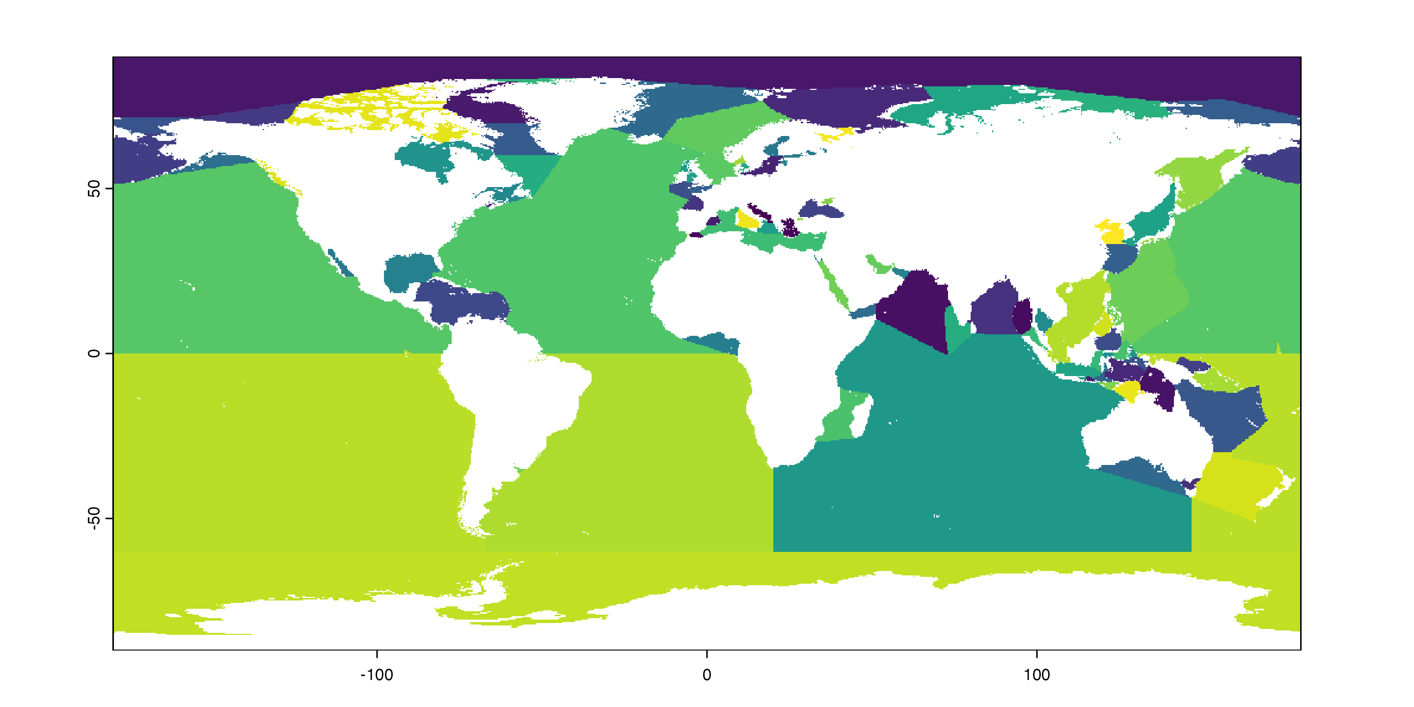
Pointers and wrapping

We’ll need to apply this grid of seas and oceans repeatedly — once for each .nc file — which means it has to get passed to all our worker cores. But it is stored as a pointer, so we can’t do that directly. We need to wrap it:

# If we don't do this it can't be passed around
# across the processes that in_parallel() will spawn
seas_zonal_wrapped <- terra::wrap(seas_zonal)

NOAA Temperature Data

Write a function very similar to the other one.

#' Process raster zonally
#'
#' Use terra to process the NCDF files
#'
#' @param fnames Vector of filenames
#' @param wrapped_seas wrapped object containing rasterized seas data
#'
#' @returns
#' @export
#'
#' @examples
process_raster_zonal <- function(fnames, wrapped_seas = seas_zonal_wrapped) {
  d <- terra::rast(fnames)
  wts <- terra::cellSize(d, unit = "km") # For scaling

  layer_varnames <- terra::varnames(d) # vector of layers
  date_seq <- rep(terra::time(d)) # vector of dates

  # New colnames for use post zonal calculation below
  new_colnames <- c("sea", paste(layer_varnames, date_seq, sep = "_"))

  # Better colnames
  tdf_seas <- d |>
    terra::rotate() |> # Convert 0 to 360 lon to -180 to +180 lon
    terra::zonal(terra::unwrap(wrapped_seas), mean, na.rm = TRUE)
  colnames(tdf_seas) <- new_colnames

  # Reshape to long
  tdf_seas |>
    tidyr::pivot_longer(
      -sea,
      names_to = c("measure", "date"),
      values_to = "value",
      names_pattern = "(.*)_(.*)"
    ) |>
    tidyr::pivot_wider(names_from = measure, values_from = value)
}

NOAA Temperature Data

Try it on one record:

process_raster_zonal(all_fnames[10000])

# A tibble: 101 × 6
   sea                    date          anom   err     ice   sst
   <chr>                  <chr>        <dbl> <dbl>   <dbl> <dbl>
 1 Adriatic Sea           2009-01-20  0.174  0.227 NaN     13.5 
 2 Aegean Sea             2009-01-20  0.796  0.146 NaN     15.9 
 3 Alboran Sea            2009-01-20 -0.692  0.168 NaN     14.8 
 4 Andaman or Burma Sea   2009-01-20 -0.548  0.124 NaN     27.1 
 5 Arabian Sea            2009-01-20  0.267  0.133 NaN     26.6 
 6 Arafura Sea            2009-01-20  0.112  0.293 NaN     29.6 
 7 Arctic Ocean           2009-01-20  0.0366 0.298   0.979 -1.74
 8 Baffin Bay             2009-01-20  0.130  0.279   0.953 -1.58
 9 Balearic (Iberian Sea) 2009-01-20  0.0595 0.130 NaN     14.0 
10 Bali Sea               2009-01-20 -0.134  0.138 NaN     28.7 
# ℹ 91 more rows

We’ll tidy the date later. You can see we get 101 summary records per day.

NOAA Temperature Data

Try it on one chunk of records:

process_raster_zonal(chunked_fnames[[1]])

# A tibble: 2,525 × 6
   sea          date         anom   err   ice   sst
   <chr>        <chr>       <dbl> <dbl> <dbl> <dbl>
 1 Adriatic Sea 1981-09-01 -0.737 0.167   NaN  23.0
 2 Adriatic Sea 1981-09-02 -0.645 0.176   NaN  23.1
 3 Adriatic Sea 1981-09-03 -0.698 0.176   NaN  22.9
 4 Adriatic Sea 1981-09-04 -0.708 0.248   NaN  22.9
 5 Adriatic Sea 1981-09-05 -1.05  0.189   NaN  22.5
 6 Adriatic Sea 1981-09-06 -1.02  0.147   NaN  22.4
 7 Adriatic Sea 1981-09-07 -0.920 0.141   NaN  22.4
 8 Adriatic Sea 1981-09-08 -0.832 0.140   NaN  22.5
 9 Adriatic Sea 1981-09-09 -0.665 0.162   NaN  22.6
10 Adriatic Sea 1981-09-10 -0.637 0.268   NaN  22.5
# ℹ 2,515 more rows

NOAA Temperature Data

Now parallelize it:

tictoc::tic("Big op")
seameans_df <- chunked_fnames |>
  map(in_parallel(
    \(x) process_raster_zonal(x),
    process_raster_zonal = process_raster_zonal,
    seas_zonal_wrapped = seas_zonal_wrapped
  )) |>
  list_rbind() |>
  mutate(
    date = ymd(date),
    year = lubridate::year(date),
    month = lubridate::month(date),
    day = lubridate::day(date),
    yrday = lubridate::yday(date),
    season = season(date)
  )
tictoc::toc()

Big op: 147.389 sec elapsed

NOAA Temperature Data

seameans_df

# A tibble: 1,622,565 × 11
   sea        date         anom   err   ice   sst  year month   day yrday season
   <chr>      <date>      <dbl> <dbl> <dbl> <dbl> <dbl> <dbl> <int> <dbl> <fct> 
 1 Adriatic … 1981-09-01 -0.737 0.167   NaN  23.0  1981     9     1   244 Summer
 2 Adriatic … 1981-09-02 -0.645 0.176   NaN  23.1  1981     9     2   245 Autumn
 3 Adriatic … 1981-09-03 -0.698 0.176   NaN  22.9  1981     9     3   246 Autumn
 4 Adriatic … 1981-09-04 -0.708 0.248   NaN  22.9  1981     9     4   247 Autumn
 5 Adriatic … 1981-09-05 -1.05  0.189   NaN  22.5  1981     9     5   248 Autumn
 6 Adriatic … 1981-09-06 -1.02  0.147   NaN  22.4  1981     9     6   249 Autumn
 7 Adriatic … 1981-09-07 -0.920 0.141   NaN  22.4  1981     9     7   250 Autumn
 8 Adriatic … 1981-09-08 -0.832 0.140   NaN  22.5  1981     9     8   251 Autumn
 9 Adriatic … 1981-09-09 -0.665 0.162   NaN  22.6  1981     9     9   252 Autumn
10 Adriatic … 1981-09-10 -0.637 0.268   NaN  22.5  1981     9    10   253 Autumn
# ℹ 1,622,555 more rows

Parallel Computing

Load the packages, as always

For example

For example: split

For example: split

For example: apply

For example: apply

For example: combine

For example: apply

How this happens

How this happens

That’s Embarrassing

That’s Embarrassing

Multicore Computing

Some Terms

Some Terms

Multicore Computing

Previously: Future and furrr

Parallel purrr

Toy Example

Toy Example

Using in_parallel()

Using in_parallel()

Extended Example

NOAA Temperature Data

NOAA Temperature Data

NOAA Temperature Data

NOAA Temperature Data

Some Prep

NOAA Temperature Data

NOAA Temperature Data

NOAA Temperature Data

NOAA Temperature Data

NOAA Temperature Data

NOAA Temperature Data

NOAA Temperature Data

Try it on one chunk of data files:

NOAA Temperature Data

NOAA Temperature Data

NOAA Temperature Data

NOAA Temperature Data

NOAA Temperature Data

Pointers and wrapping

NOAA Temperature Data

NOAA Temperature Data

NOAA Temperature Data

NOAA Temperature Data

NOAA Temperature Data

NOAA that’s more like it

Parallel `purrr`

Using `in_parallel()`

Using `in_parallel()`