Example 09: Databases and APIs

── Attaching core tidyverse packages ──────────────────────── tidyverse 2.0.0 ──
✔ dplyr     1.2.1     ✔ readr     2.2.0
✔ forcats   1.0.1     ✔ stringr   1.6.0
✔ ggplot2   4.0.3     ✔ tibble    3.3.1
✔ lubridate 1.9.5     ✔ tidyr     1.3.2
✔ purrr     1.2.2     
── Conflicts ────────────────────────────────────────── tidyverse_conflicts() ──
✖ dplyr::filter() masks stats::filter()
✖ dplyr::lag()    masks stats::lag()
ℹ Use the conflicted package (<http://conflicted.r-lib.org/>) to force all conflicts to become errors
here() starts at /Users/kjhealy/Documents/courses/mptc

Working with
`tidycensus`

Load our packages

library(here)       # manage file paths
library(socviz)     # data and some useful things, especially %notin%
library(tidyverse)  # your friend and mine

library(scales)     # Convenient scale labels


Attaching package: 'scales'

The following object is masked from 'package:purrr':

    discard

The following object is masked from 'package:readr':

    col_factor

library(tidycensus) # Tidily talk to the Census
library(sf)         # Draw maps with ggplot

Linking to GEOS 3.13.0, GDAL 3.8.5, PROJ 9.5.1; sf_use_s2() is TRUE

# Don't needlessly download geometries files multiple times
options(tigris_use_cache = TRUE)

Census Data

Make sure you have a Census API key. Load it after you load tidycensus

library(tidycensus)

census_api_key("1234567890987654321")

Get one from https://api.census.gov/data/key_signup.html

Decennial Census Variables

There are a lot of them:

census_vars <- load_variables(year = 2010,
                              dataset = "sf1",
                              cache = TRUE)

Warning: `cache` is deprecated and ignored. tidycensus no longer writes
variable metadata to a local cache.

census_vars

# A tibble: 8,959 × 3
   name    label                                concept         
   <chr>   <chr>                                <chr>           
 1 H001001 Total                                HOUSING UNITS   
 2 H002001 Total                                URBAN AND RURAL 
 3 H002002 Total!!Urban                         URBAN AND RURAL 
 4 H002003 Total!!Urban!!Inside urbanized areas URBAN AND RURAL 
 5 H002004 Total!!Urban!!Inside urban clusters  URBAN AND RURAL 
 6 H002005 Total!!Rural                         URBAN AND RURAL 
 7 H002006 Total!!Not defined for this file     URBAN AND RURAL 
 8 H003001 Total                                OCCUPANCY STATUS
 9 H003002 Total!!Occupied                      OCCUPANCY STATUS
10 H003003 Total!!Vacant                        OCCUPANCY STATUS
# ℹ 8,949 more rows

Median Age by State:

age10 <- get_decennial(geography = "state",
                       variables = "P013001",
                       year = 2010)

Getting data from the 2010 decennial Census

Using Census Summary File 1

age10

# A tibble: 52 × 4
   GEOID NAME        variable value
   <chr> <chr>       <chr>    <dbl>
 1 01    Alabama     P013001   37.9
 2 02    Alaska      P013001   33.8
 3 04    Arizona     P013001   35.9
 4 05    Arkansas    P013001   37.4
 5 06    California  P013001   35.2
 6 22    Louisiana   P013001   35.8
 7 21    Kentucky    P013001   38.1
 8 08    Colorado    P013001   36.1
 9 09    Connecticut P013001   40  
10 10    Delaware    P013001   38.8
# ℹ 42 more rows

Some County Data for North Carolina

# Census variable names
popvars <- c("P005003", "P005004", "P005006", "P004003")


# Get a county-level dataset for NC with these variables
# The summary value is the total population.
nc <- get_decennial(geography = "county",
                    variables = popvars,
                    year = 2010,
                    summary_var = "P001001",
                    state = "NC") |>
  mutate(pct = 100 * (value / summary_value))

Getting data from the 2010 decennial Census

Using Census Summary File 1

nc

# A tibble: 400 × 6
   GEOID NAME                             variable  value summary_value   pct
   <chr> <chr>                            <chr>     <dbl>         <dbl> <dbl>
 1 37007 Anson County, North Carolina     P005003   12344         26948  45.8
 2 37011 Avery County, North Carolina     P005003   16029         17797  90.1
 3 37003 Alexander County, North Carolina P005003   32671         37198  87.8
 4 37015 Bertie County, North Carolina    P005003    7393         21282  34.7
 5 37013 Beaufort County, North Carolina  P005003   31705         47759  66.4
 6 37005 Alleghany County, North Carolina P005003    9862         11155  88.4
 7 37001 Alamance County, North Carolina  P005003  101718        151131  67.3
 8 37009 Ashe County, North Carolina      P005003   25420         27281  93.2
 9 37017 Bladen County, North Carolina    P005003   19242         35190  54.7
10 37019 Brunswick County, North Carolina P005003   86818        107431  80.8
# ℹ 390 more rows

We can do this a little more elegantly:

# Census variable names
popvars <- tribble(
  ~variable, ~name,
  "P005003", "nh_white",
  "P005004", "nh_black",
  "P005006", "nh_asian",
  "P004003", "hispanic")

popvars

# A tibble: 4 × 2
  variable name    
  <chr>    <chr>   
1 P005003  nh_white
2 P005004  nh_black
3 P005006  nh_asian
4 P004003  hispanic

# Get a county-level dataset for NC with these variables
# The summary value is the total population.
nc <- get_decennial(geography = "county",
                    variables = popvars$variable, 
                    year = 2010,
                    summary_var = "P001001",
                    state = "NC") |>
  mutate(pct = 100 * (value / summary_value))

Getting data from the 2010 decennial Census

Using Census Summary File 1

nc

# A tibble: 400 × 6
   GEOID NAME                             variable  value summary_value   pct
   <chr> <chr>                            <chr>     <dbl>         <dbl> <dbl>
 1 37007 Anson County, North Carolina     P005003   12344         26948  45.8
 2 37011 Avery County, North Carolina     P005003   16029         17797  90.1
 3 37003 Alexander County, North Carolina P005003   32671         37198  87.8
 4 37015 Bertie County, North Carolina    P005003    7393         21282  34.7
 5 37013 Beaufort County, North Carolina  P005003   31705         47759  66.4
 6 37005 Alleghany County, North Carolina P005003    9862         11155  88.4
 7 37001 Alamance County, North Carolina  P005003  101718        151131  67.3
 8 37009 Ashe County, North Carolina      P005003   25420         27281  93.2
 9 37017 Bladen County, North Carolina    P005003   19242         35190  54.7
10 37019 Brunswick County, North Carolina P005003   86818        107431  80.8
# ℹ 390 more rows

nc |>
  left_join(popvars, by = "variable") |>
  relocate(name, .after = variable) |>
  select(-variable) |>
  pivot_wider(names_from = name,
              names_glue = "{name}_{.value}",
              values_from = c(value, pct)) |>
  mutate(NAME = str_remove(NAME, " County.*"))

# A tibble: 100 × 11
   GEOID NAME      summary_value nh_white_value nh_black_value nh_asian_value
   <chr> <chr>             <dbl>          <dbl>          <dbl>          <dbl>
 1 37007 Anson             26948          12344          13038            281
 2 37011 Avery             17797          16029            706             56
 3 37003 Alexander         37198          32671           2025            357
 4 37015 Bertie            21282           7393          13252            103
 5 37013 Beaufort          47759          31705          12105            158
 6 37005 Alleghany         11155           9862            133             53
 7 37001 Alamance         151131         101718          27985           1806
 8 37009 Ashe              27281          25420            148            105
 9 37017 Bladen            35190          19242          12202             67
10 37019 Brunswick        107431          86818          12120            560
# ℹ 90 more rows
# ℹ 5 more variables: hispanic_value <dbl>, nh_white_pct <dbl>,
#   nh_black_pct <dbl>, nh_asian_pct <dbl>, hispanic_pct <dbl>

Put it in an object:

Now we have:

nc_wide

# A tibble: 100 × 11
   GEOID NAME      summary_value nh_white_value nh_black_value nh_asian_value
   <chr> <chr>             <dbl>          <dbl>          <dbl>          <dbl>
 1 37007 Anson             26948          12344          13038            281
 2 37011 Avery             17797          16029            706             56
 3 37003 Alexander         37198          32671           2025            357
 4 37015 Bertie            21282           7393          13252            103
 5 37013 Beaufort          47759          31705          12105            158
 6 37005 Alleghany         11155           9862            133             53
 7 37001 Alamance         151131         101718          27985           1806
 8 37009 Ashe              27281          25420            148            105
 9 37017 Bladen            35190          19242          12202             67
10 37019 Brunswick        107431          86818          12120            560
# ℹ 90 more rows
# ℹ 5 more variables: hispanic_value <dbl>, nh_white_pct <dbl>,
#   nh_black_pct <dbl>, nh_asian_pct <dbl>, hispanic_pct <dbl>

Top 20 Counties by Percent Hispanic

nc_wide |>
  slice_max(order_by = hispanic_pct, n = 20) |>
  ggplot(mapping = aes(x = hispanic_pct,
                       y = reorder(NAME, hispanic_pct))) +
  geom_point() +
  labs(x = "Percent Hispanic",
       y = NULL,
       title = "North Carolina Counties")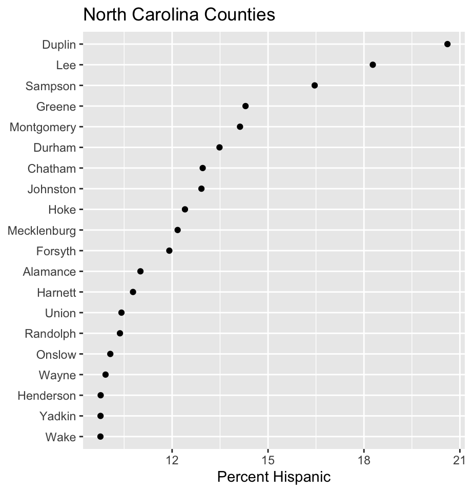

Log population vs Percent Hispanic

nc_wide |>
  ggplot(mapping = aes(x = summary_value,
                       y = hispanic_pct)) +
  geom_point() +
  scale_x_log10(labels = label_number(scale_cut = cut_short_scale())) +
  labs(x = "Log Population",
       y = "Percent Hispanic",
       title = "North Carolina Counties")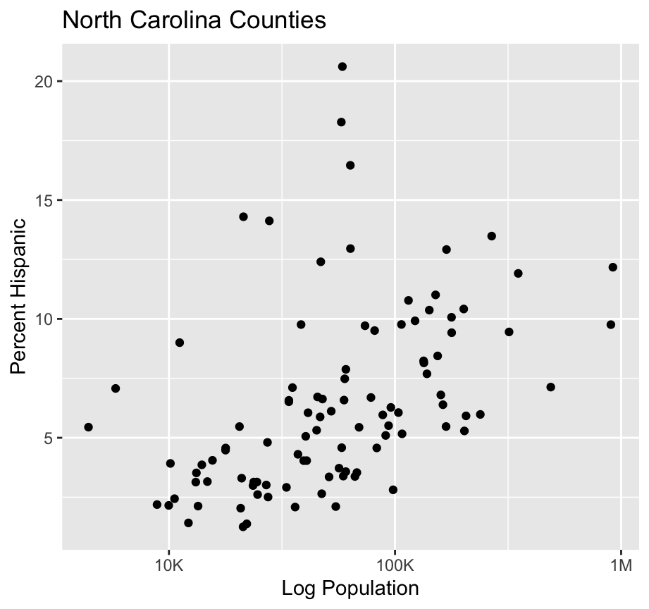

Log population vs Percent Black

nc_wide |>
  ggplot(mapping = aes(x = summary_value,
                       y = nh_black_pct)) +
  geom_point() +
  scale_x_log10(labels = label_number(scale_cut = cut_short_scale())) +
  labs(x = "Log Population",
       y = "Percent Black",
       title = "North Carolina Counties")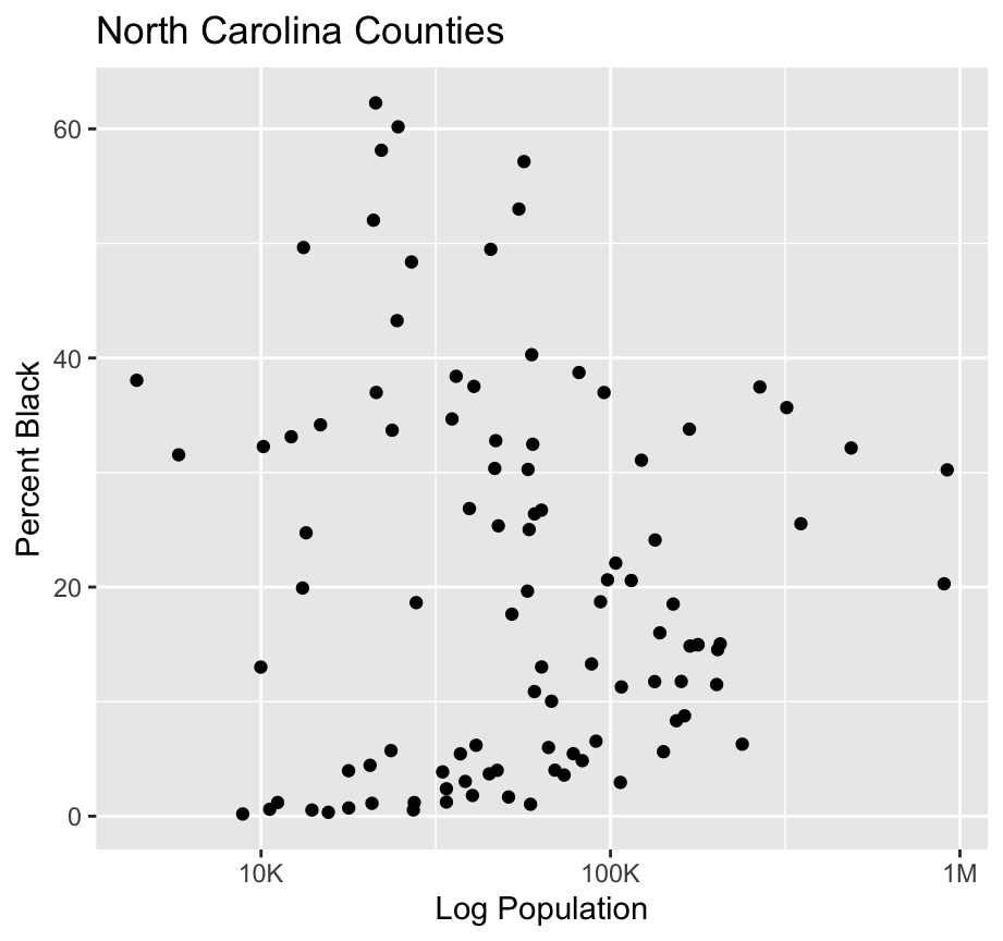

Percent White vs Percent Black

nc_wide |>
  ggplot(mapping = aes(x = nh_white_pct,
                       y = nh_black_pct)) +
  geom_point() +
  labs(x = "Percent White",
       y = "Percent Black",
       title = "North Carolina Counties")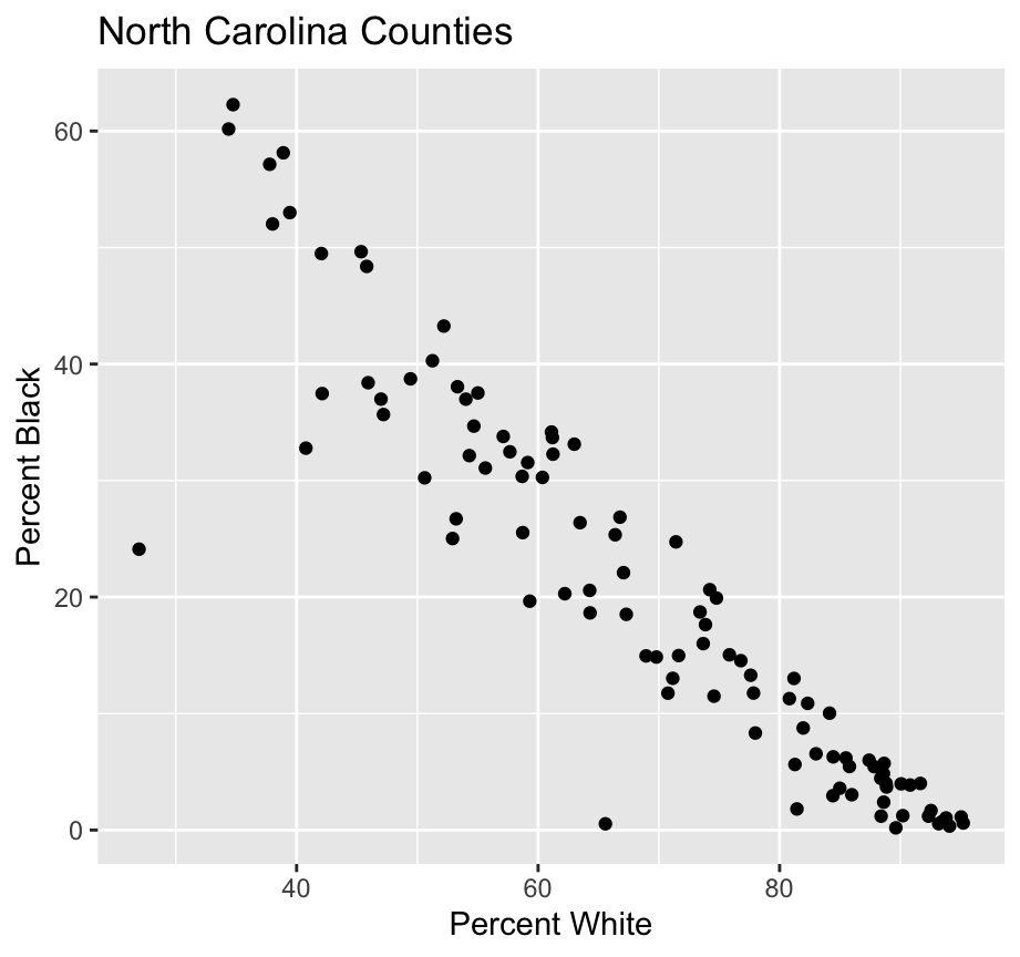

Population Pyramids

We can ask the Census for its estimates of the age breakdown of the population, using the get_estimates() function.

usa <- get_estimates(
    geography = "us",
    product = "characteristics",
    breakdown = c("SEX", "AGEGROUP"),
    breakdown_labels = TRUE,
    year = 2019
  )

usa

# A tibble: 96 × 5
   GEOID NAME              value SEX        AGEGROUP          
   <chr> <chr>             <dbl> <chr>      <fct>             
 1 1     United States 328239523 Both sexes All ages          
 2 1     United States  19576683 Both sexes Age 0 to 4 years  
 3 1     United States  20195895 Both sexes Age 5 to 9 years  
 4 1     United States 161657324 Male       All ages          
 5 1     United States  10009207 Male       Age 0 to 4 years  
 6 1     United States  10322762 Male       Age 5 to 9 years  
 7 1     United States 166582199 Female     All ages          
 8 1     United States   9567476 Female     Age 0 to 4 years  
 9 1     United States   7528626 Female     Age 70 to 74 years
10 1     United States  20798268 Both sexes Age 10 to 14 years
# ℹ 86 more rows

Population Pyramids

usa_pyr <- usa |>
  filter(AGEGROUP %notin% "All ages",
         str_detect(AGEGROUP, "Age"),
         SEX %notin% "Both sexes") |>
  mutate(value = ifelse(SEX == "Male", -value, value))

usa_pyr

# A tibble: 36 × 5
   GEOID NAME              value SEX    AGEGROUP          
   <chr> <chr>             <dbl> <chr>  <fct>             
 1 1     United States -10009207 Male   Age 0 to 4 years  
 2 1     United States -10322762 Male   Age 5 to 9 years  
 3 1     United States   9567476 Female Age 0 to 4 years  
 4 1     United States   7528626 Female Age 70 to 74 years
 5 1     United States   9873133 Female Age 5 to 9 years  
 6 1     United States -10618261 Male   Age 10 to 14 years
 7 1     United States  10180007 Female Age 10 to 14 years
 8 1     United States -11064752 Male   Age 20 to 24 years
 9 1     United States  10568188 Female Age 20 to 24 years
10 1     United States -12004570 Male   Age 25 to 29 years
# ℹ 26 more rows

Default:

usa_pyr |>
  ggplot(mapping = aes(x = value,
                       y = AGEGROUP,
                       fill = SEX)) +
  geom_col(width = 0.95, alpha = 0.75) +
  labs(x = "Count",
       y = NULL,
       title = "US Population Pyramid")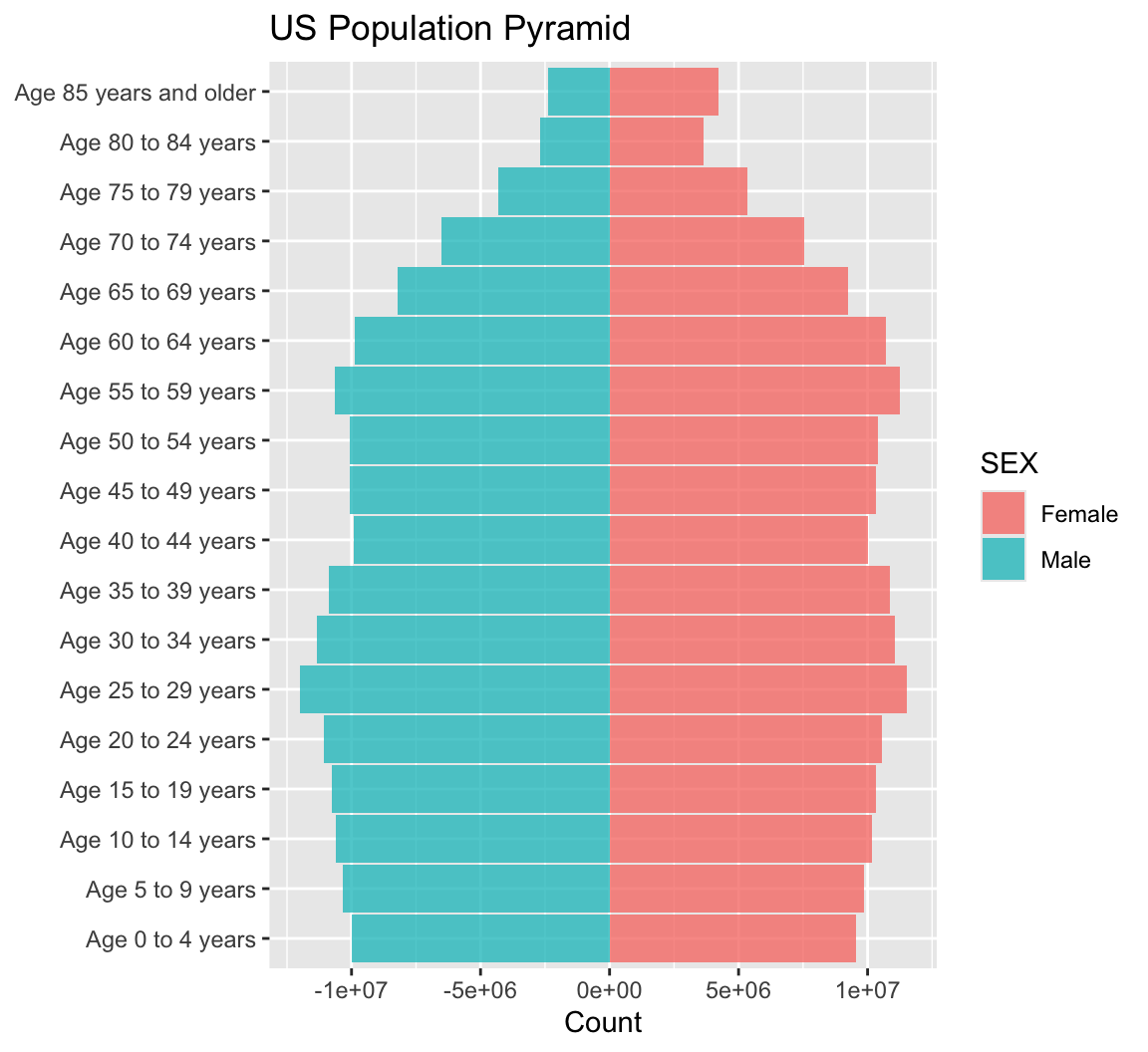

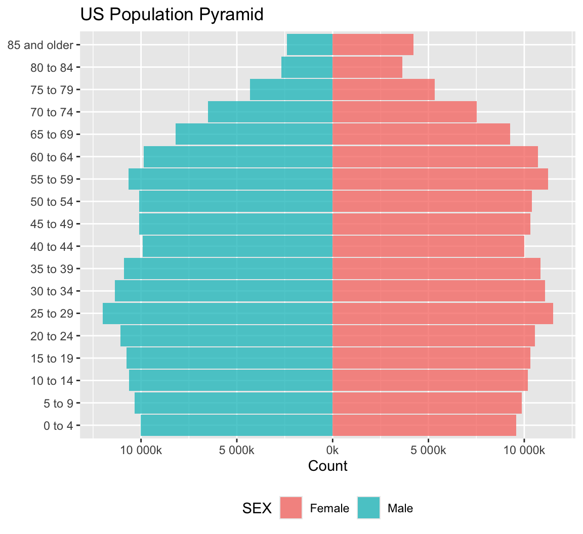
Fix the scales:

usa_pyr |>
  ggplot(mapping = aes(x = value,
                       y = AGEGROUP,
                       fill = SEX)) +
  geom_col(width = 0.95, alpha = 0.75) +
  # In the two scale functions we use \(x) label_number()
  # and \(x) str_remove_all() as anonymous functions.
  scale_x_continuous(
    labels = \(x) label_number(scale = 0.001, suffix = "k")(abs(x))) +
  scale_y_discrete(
    labels = \(x) str_remove_all(x, "Age | years")) +
  labs(x = "Count",
       y = NULL,
       title= "US Population Pyramid") +
  theme(legend.position = "bottom")

Working with tidycensus

Load our packages

Census Data

Decennial Census Variables

Some County Data for North Carolina

Top 20 Counties by Percent Hispanic

Log population vs Percent Hispanic

Log population vs Percent Black

Percent White vs Percent Black

Population Pyramids

Population Pyramids

Working with
`tidycensus`