library(tidyverse)
library(socviz)
library(gapminder)
library(here)Example 04: R and ggplot basics
We begin as usual by loading the tidyverse package and a few others.
How R thinks
To start, we can say: in R, everything has a name and everything is an object. You do things to named objects with functions (which are themselves objects!). And you create an object by assigning a thing to a name.
Assignment is the act of attaching a thing to a name. It is represented by <- or = and you can read it as “gets” or “is”. Type it by with the < and then the - key. Better, there is a shortcut: on Mac OS it is Option - or Option and the - (minus or hyphen) key together. On Windows it’s Alt -.
Objects
We’re going to use the c() function (c for concatenate) to stick some numbers together into a vector. And we will assign that the name my_numbers.
## Inside code chunks, lines beginning with a # character are comments
## Comments are ignored by R

my_numbers <- c(1, 1, 2, 4, 1, 3, 1, 5) # Anything after a # character is ignored as well

## Now we have an object by this name
my_numbers
[1] 1 1 2 4 1 3 1 5Again, in that previous chunk we created an object by assigning something (the result of a function) to a name. Now that thing exists in our project environment.
my_numbers[1] 1 1 2 4 1 3 1 5R has a few built-in objects.
letters [1] "a" "b" "c" "d" "e" "f" "g" "h" "i" "j" "k" "l" "m" "n" "o" "p" "q" "r" "s"
[20] "t" "u" "v" "w" "x" "y" "z"LETTERS [1] "A" "B" "C" "D" "E" "F" "G" "H" "I" "J" "K" "L" "M" "N" "O" "P" "Q" "R" "S"
[20] "T" "U" "V" "W" "X" "Y" "Z"pi[1] 3.141593But mostly we will be creating objects.
R is a calculator
You don’t have to make objects. You can just treat R like a calculator that spits out answers at the console.
(31 * 12) / 2^4[1] 23.25sqrt(25)[1] 5log(100)[1] 4.60517log10(100)[1] 2The commands that look like this() are called functions.
But everything you do along these lines can, if you want, be assigned to a name. Like my_five <- sqrt(25).
You can do logic
4 < 10[1] TRUE4 > 2 & 1 > 0.5 # The "&" means "and"[1] TRUE4 < 2 | 1 > 0.5 # The "|" means "or"[1] TRUE4 < 2 | 1 < 0.5[1] FALSEA logical test:
2 == 2 # Write `=` twice[1] TRUENot this:
## This will cause an error, because R will think you are trying to assign a value
2 = 2

## Error in 2 = 2 : invalid (do_set) left-hand side to assignment
Testing for “not equal to” or “is not”:
3 != 7 # Write `!` and then `=` to make `!=`[1] TRUEMore about objects
my_numbers # We created this a few minutes ago[1] 1 1 2 4 1 3 1 5letters # This one is built-in [1] "a" "b" "c" "d" "e" "f" "g" "h" "i" "j" "k" "l" "m" "n" "o" "p" "q" "r" "s"
[20] "t" "u" "v" "w" "x" "y" "z"pi # Also built-in[1] 3.141593Creating objects: assign a thing (usually the result of a function) to a name.
## this object... gets ... the output of this function
my_numbers <- c(1, 2, 3, 1, 3, 5, 25, 10)

your_numbers <- c(5, 31, 71, 1, 3, 21, 6, 52)
You do things with functions
Functions usually take input, perform actions, and then return output.
# Calculate the mean of my_numbers with the mean() function
mean(x = my_numbers)
[1] 6.25The instructions you can give a function are its arguments. Here, x is saying “this is the thing I want you to take the mean of”.
If you provide arguments in the “right” order (the order the function expects), you don’t have to name them.
mean(my_numbers)[1] 6.25Look at the help for mean() with ?mean to learn what trim is doing.
## The sample() function
x <- sample(x = 1:100, size = 100, replace = TRUE) # What does each piece do here?
mean(x)
[1] 48.71mean(x, trim = 0.1)[1] 47.9375For functions with more than one or two arguments, explicitly naming arguments is good practice, especially when learning the language.
Data
Built-in datasets
A few datasets come built-in, for convenience. Here is one:
mtcars mpg cyl disp hp drat wt qsec vs am gear carb
Mazda RX4 21.0 6 160.0 110 3.90 2.620 16.46 0 1 4 4
Mazda RX4 Wag 21.0 6 160.0 110 3.90 2.875 17.02 0 1 4 4
Datsun 710 22.8 4 108.0 93 3.85 2.320 18.61 1 1 4 1
Hornet 4 Drive 21.4 6 258.0 110 3.08 3.215 19.44 1 0 3 1
Hornet Sportabout 18.7 8 360.0 175 3.15 3.440 17.02 0 0 3 2
Valiant 18.1 6 225.0 105 2.76 3.460 20.22 1 0 3 1
Duster 360 14.3 8 360.0 245 3.21 3.570 15.84 0 0 3 4
Merc 240D 24.4 4 146.7 62 3.69 3.190 20.00 1 0 4 2
Merc 230 22.8 4 140.8 95 3.92 3.150 22.90 1 0 4 2
Merc 280 19.2 6 167.6 123 3.92 3.440 18.30 1 0 4 4
Merc 280C 17.8 6 167.6 123 3.92 3.440 18.90 1 0 4 4
Merc 450SE 16.4 8 275.8 180 3.07 4.070 17.40 0 0 3 3
Merc 450SL 17.3 8 275.8 180 3.07 3.730 17.60 0 0 3 3
Merc 450SLC 15.2 8 275.8 180 3.07 3.780 18.00 0 0 3 3
Cadillac Fleetwood 10.4 8 472.0 205 2.93 5.250 17.98 0 0 3 4
Lincoln Continental 10.4 8 460.0 215 3.00 5.424 17.82 0 0 3 4
Chrysler Imperial 14.7 8 440.0 230 3.23 5.345 17.42 0 0 3 4
Fiat 128 32.4 4 78.7 66 4.08 2.200 19.47 1 1 4 1
Honda Civic 30.4 4 75.7 52 4.93 1.615 18.52 1 1 4 2
Toyota Corolla 33.9 4 71.1 65 4.22 1.835 19.90 1 1 4 1
Toyota Corona 21.5 4 120.1 97 3.70 2.465 20.01 1 0 3 1
Dodge Challenger 15.5 8 318.0 150 2.76 3.520 16.87 0 0 3 2
AMC Javelin 15.2 8 304.0 150 3.15 3.435 17.30 0 0 3 2
Camaro Z28 13.3 8 350.0 245 3.73 3.840 15.41 0 0 3 4
Pontiac Firebird 19.2 8 400.0 175 3.08 3.845 17.05 0 0 3 2
Fiat X1-9 27.3 4 79.0 66 4.08 1.935 18.90 1 1 4 1
Porsche 914-2 26.0 4 120.3 91 4.43 2.140 16.70 0 1 5 2
Lotus Europa 30.4 4 95.1 113 3.77 1.513 16.90 1 1 5 2
Ford Pantera L 15.8 8 351.0 264 4.22 3.170 14.50 0 1 5 4
Ferrari Dino 19.7 6 145.0 175 3.62 2.770 15.50 0 1 5 6
Maserati Bora 15.0 8 301.0 335 3.54 3.570 14.60 0 1 5 8
Volvo 142E 21.4 4 121.0 109 4.11 2.780 18.60 1 1 4 2Some packages also come with datasets. The socviz package has a few. The mpg dataset is a kind of updated version of the mtcars dataset.
mpg# A tibble: 234 × 11
manufacturer model displ year cyl trans drv cty hwy fl class
<chr> <chr> <dbl> <int> <int> <chr> <chr> <int> <int> <chr> <chr>
1 audi a4 1.8 1999 4 auto… f 18 29 p comp…
2 audi a4 1.8 1999 4 manu… f 21 29 p comp…
3 audi a4 2 2008 4 manu… f 20 31 p comp…
4 audi a4 2 2008 4 auto… f 21 30 p comp…
5 audi a4 2.8 1999 6 auto… f 16 26 p comp…
6 audi a4 2.8 1999 6 manu… f 18 26 p comp…
7 audi a4 3.1 2008 6 auto… f 18 27 p comp…
8 audi a4 quattro 1.8 1999 4 manu… 4 18 26 p comp…
9 audi a4 quattro 1.8 1999 4 auto… 4 16 25 p comp…
10 audi a4 quattro 2 2008 4 manu… 4 20 28 p comp…
# ℹ 224 more rowsLike functions that are come in packages, you don’t see built-in or packaged datasets in your object inspector (because you did not create them yourself in your session), but they are accessible to you. If you want to make a copy of one of these datasets to inspect, you can assign it to a name:
my_mpg <- mpgNow you’ll see it in your object inspector.
Reading in data
The most common way to get data into R is to read it from a file. The readr package (part of the tidyverse) has functions for reading in data files. The most common kind of data file is a comma-separated values (CSV) file. We read it in with read_csv(). We describe a file path relative to the project root, with the help of the here() function from the here package.
organs <- read_csv(here("data", "organdonation.csv"))Rows: 238 Columns: 21
── Column specification ────────────────────────────────────────────────────────
Delimiter: ","
chr (7): country, world, opt, consent.law, consent.practice, consistent, ccode
dbl (14): year, donors, pop, pop.dens, gdp, gdp.lag, health, health.lag, pub...
ℹ Use `spec()` to retrieve the full column specification for this data.
ℹ Specify the column types or set `show_col_types = FALSE` to quiet this message.organs# A tibble: 238 × 21
country year donors pop pop.dens gdp gdp.lag health health.lag pubhealth
<chr> <dbl> <dbl> <dbl> <dbl> <dbl> <dbl> <dbl> <dbl> <dbl>
1 Austra… NA NA 17065 0.220 16774 16591 1300 1224 4.8
2 Austra… 1991 12.1 17284 0.223 17171 16774 1379 1300 5.4
3 Austra… 1992 12.4 17495 0.226 17914 17171 1455 1379 5.4
4 Austra… 1993 12.5 17667 0.228 18883 17914 1540 1455 5.4
5 Austra… 1994 10.2 17855 0.231 19849 18883 1626 1540 5.4
6 Austra… 1995 10.2 18072 0.233 21079 19849 1737 1626 5.5
7 Austra… 1996 10.6 18311 0.237 21923 21079 1846 1737 5.6
8 Austra… 1997 10.3 18518 0.239 22961 21923 1948 1846 5.7
9 Austra… 1998 10.5 18711 0.242 24148 22961 2077 1948 5.9
10 Austra… 1999 8.67 18926 0.244 25445 24148 2231 2077 6.1
# ℹ 228 more rows
# ℹ 11 more variables: roads <dbl>, cerebvas <dbl>, assault <dbl>,
# external <dbl>, txp.pop <dbl>, world <chr>, opt <chr>, consent.law <chr>,
# consent.practice <chr>, consistent <chr>, ccode <chr>ggplot basics
To draw a graph in ggplot requires two kinds of statements: one saying what the data is and what relationship we want to plot, and the second saying what kind of plot we want. The first one is done by the ggplot() function.
ggplot(data = mpg,
       mapping = aes(x = displ, y = hwy))
You can see that by itself it doesn’t do anything.
But if we add a function saying what kind of plot, we get a result:
ggplot(data = mpg,
       mapping = aes(x = displ, y = hwy)) +
  geom_point()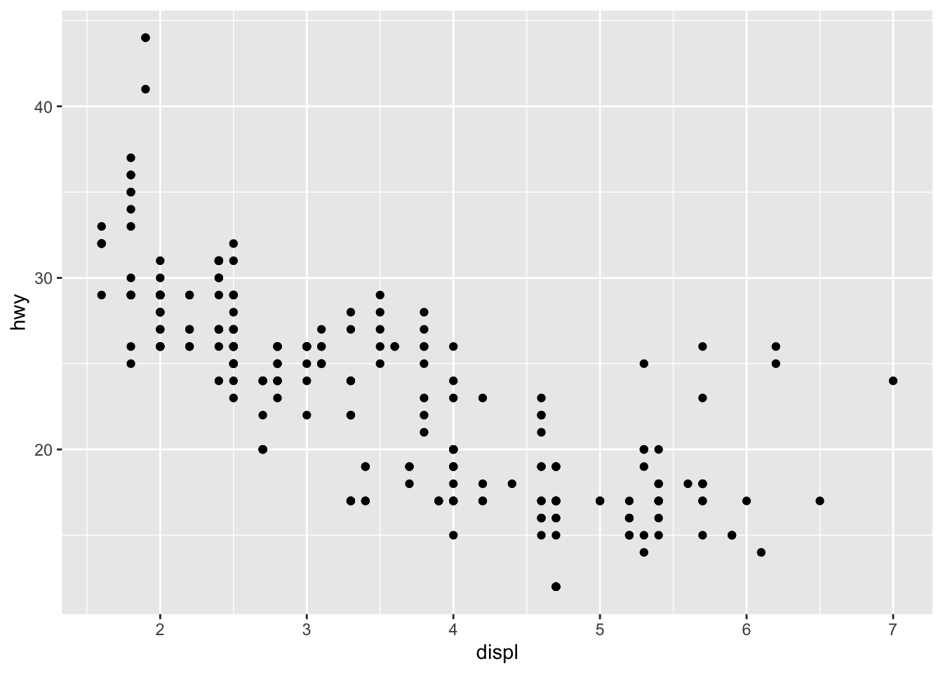
The data argument says which table of data to use. The mapping argument, which is done using the “aesthetic” function aes() tells ggplot which visual elements on the plot will represent which columns or variables in the data.
# The gapminder data
library(gapminder)
gapminder
# A tibble: 1,704 × 6
country continent year lifeExp pop gdpPercap
<fct> <fct> <int> <dbl> <int> <dbl>
1 Afghanistan Asia 1952 28.8 8425333 779.
2 Afghanistan Asia 1957 30.3 9240934 821.
3 Afghanistan Asia 1962 32.0 10267083 853.
4 Afghanistan Asia 1967 34.0 11537966 836.
5 Afghanistan Asia 1972 36.1 13079460 740.
6 Afghanistan Asia 1977 38.4 14880372 786.
7 Afghanistan Asia 1982 39.9 12881816 978.
8 Afghanistan Asia 1987 40.8 13867957 852.
9 Afghanistan Asia 1992 41.7 16317921 649.
10 Afghanistan Asia 1997 41.8 22227415 635.
# ℹ 1,694 more rowsA histogram is a summary of the distribution of a single variable:
ggplot(data = gapminder,
       mapping = aes(x = lifeExp)) +
  geom_histogram()
`stat_bin()` using `bins = 30`. Pick better value `binwidth`.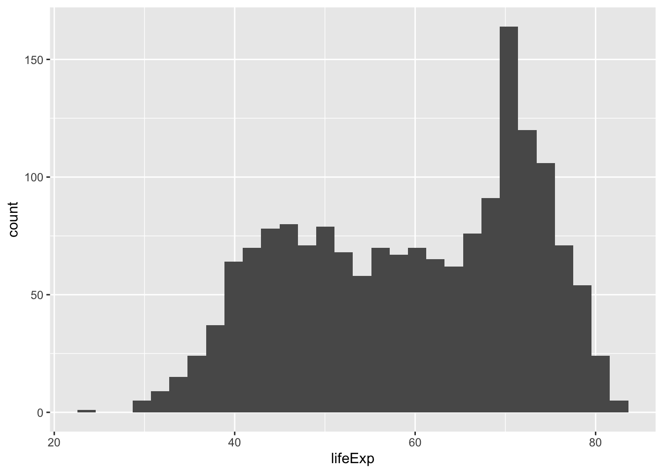
A scatterplot shows how two variables co-vary:
ggplot(data = gapminder,
       mapping = aes(x = gdpPercap, y = lifeExp)) +
  geom_point()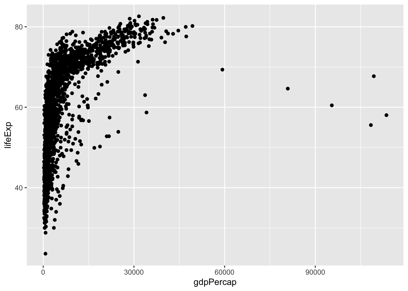
A boxplot is another way of showing the distribution of a single variable:
ggplot(data = gapminder,
       mapping = aes(y = lifeExp)) +
  geom_boxplot()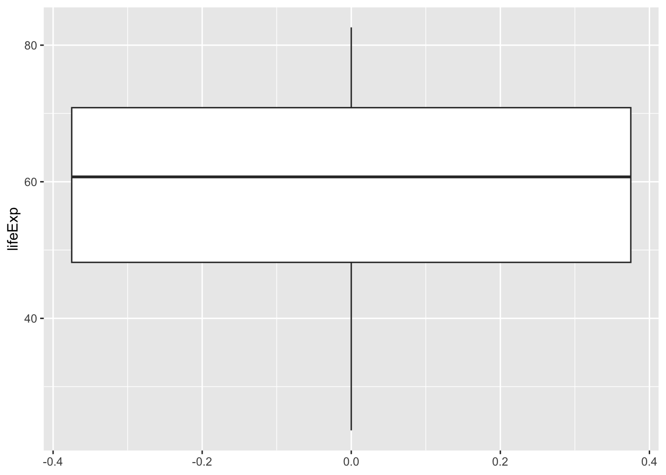
Boxplots are much more useful if we compare several of them:
ggplot(data = gapminder,
       mapping = aes(x = continent, y = lifeExp)) +
  geom_boxplot()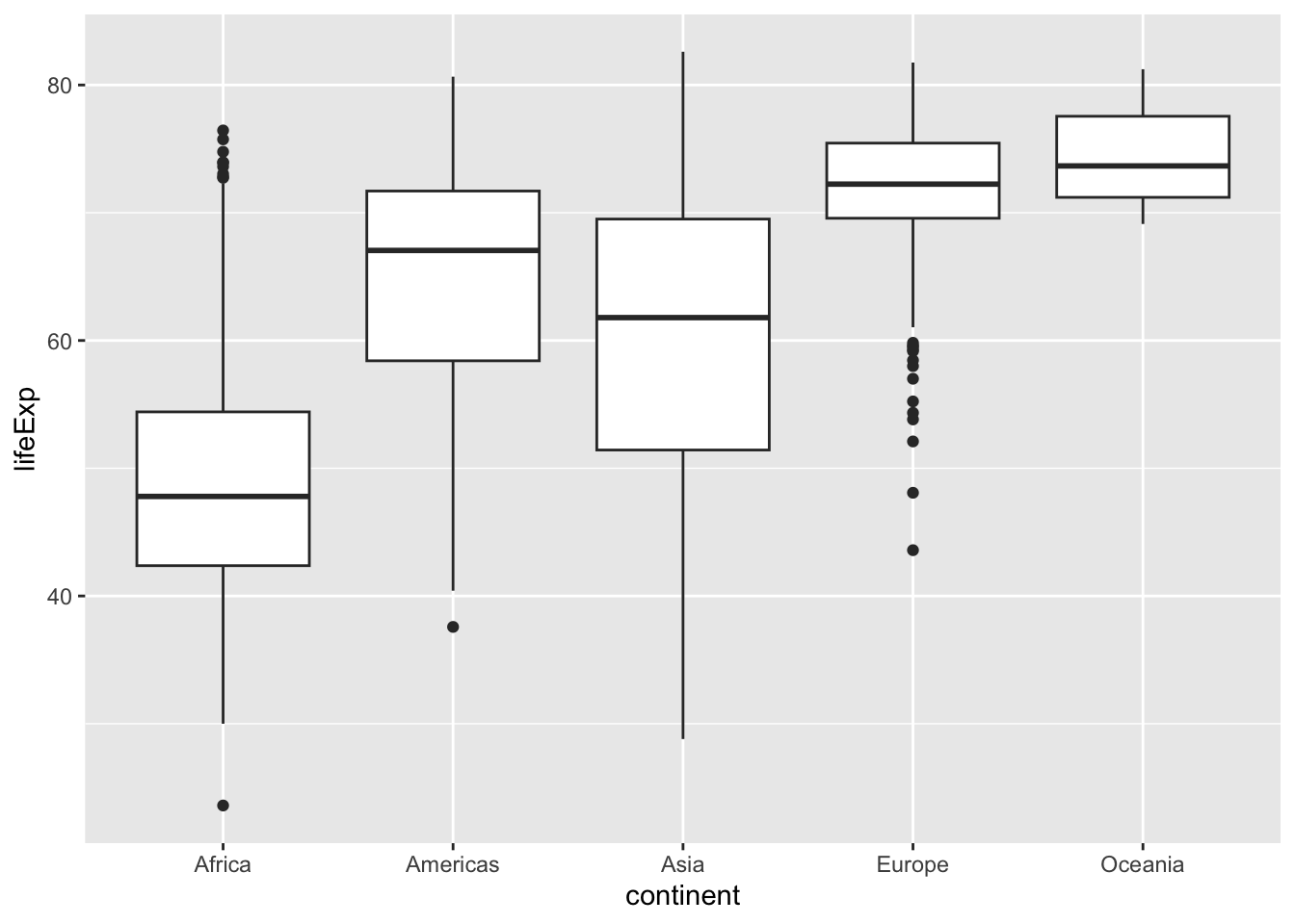
Faceting
Faceting is a powerful way to make “small multiples”, where we make the same plot for different subsets of the data.
gapminder |>
  ggplot(mapping = aes(x = year,
                       y = gdpPercap)) +
  geom_line()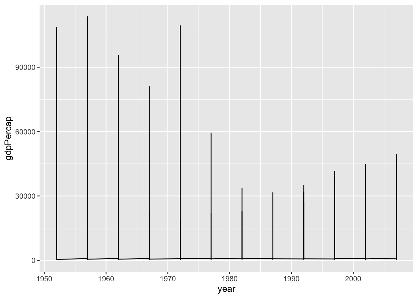
That looks weird. What has gone wrong? Remember, ggplot only knows about the relationships you tell it about. Our data are country-years and we have asked it to draw a line graph using Year and GDP per capita. And that is what it’s done. But it doesn’t know anything about the country-level structure of the data. So the geom_line() function is trying to connect all the points in the dataset in a single line, which is not what we want. We want to connect the points for each country separately. We do that by telling geom_line() to group the data by country:
gapminder |>
  ggplot(mapping = aes(x = year,
                       y = gdpPercap)) +
  geom_line(mapping = aes(group = country))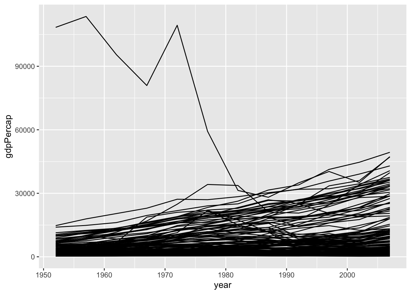
Think of the group aesthetic as telling ggplot which points belong together, or when to “lift the pen” when drawing lines.
Facet to make small multiples:
gapminder |>
  ggplot(mapping =
           aes(x = year,
           y = gdpPercap)) +
  geom_line(mapping = aes(group = country)) +
  facet_wrap(~ continent)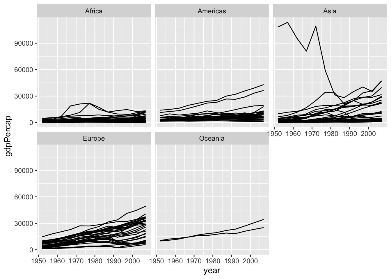
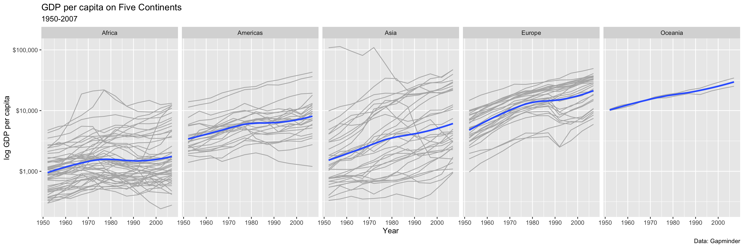
p <- ggplot(data = gapminder,
            mapping = aes(x = year,
                          y = gdpPercap))

p_out <- p + geom_line(color="gray70",
              mapping=aes(group = country)) +
    geom_smooth(linewidth = 1.1,
                method = "loess",
                se = FALSE) +
    scale_y_log10(labels=scales::label_dollar()) +
    facet_wrap(~ continent, ncol = 5) +
    labs(x = "Year",
         y = "log GDP per capita",
         title = "GDP per capita on Five Continents",
         subtitle = "1950-2007",
         caption = "Data: Gapminder")

p_out
`geom_smooth()` using formula = 'y ~ x'