Example 09: Functions and Iteration

── Attaching core tidyverse packages ──────────────────────── tidyverse 2.0.0 ──
✔ dplyr     1.1.4     ✔ readr     2.1.5
✔ forcats   1.0.1     ✔ stringr   1.5.2
✔ ggplot2   4.0.0     ✔ tibble    3.3.0
✔ lubridate 1.9.4     ✔ tidyr     1.3.1
✔ purrr     1.1.0     
── Conflicts ────────────────────────────────────────── tidyverse_conflicts() ──
✖ dplyr::filter() masks stats::filter()
✖ dplyr::lag()    masks stats::lag()
ℹ Use the conflicted package (<http://conflicted.r-lib.org/>) to force all conflicts to become errors
here() starts at /Users/kjhealy/Documents/courses/mptc

library(broom)

Functions

my_adder <- function(x, add = 1) {
  x + add
}

my_adder(10)

[1] 11

my_adder(1:10)

 [1]  2  3  4  5  6  7  8  9 10 11

# This won't work
# my_adder("a")

Guard clauses and error handling:

my_adder <- function(x, add = 1) {
  if(!is.numeric(x)) {
    return("Argument `x` must be numeric.")
  }

  x + add
}

my_adder("a")

[1] "Argument `x` must be numeric."

my_adder <- function(x, add = 1) {
  if(!is.numeric(x)) {
    return("Argument `x` must be numeric.")
  }

  if(!is.numeric(add)) {
    return("Argument `add` must be numeric.")
  }

  x + add
}

Here I use return() in the guard clauses in order to make this example work as part of the pipeline that creates the site. But really I should use stop().

my_adder(1:10, 5)

 [1]  6  7  8  9 10 11 12 13 14 15

my_adder(1:10, "c")

[1] "Argument `add` must be numeric."

Elvis PCA Example

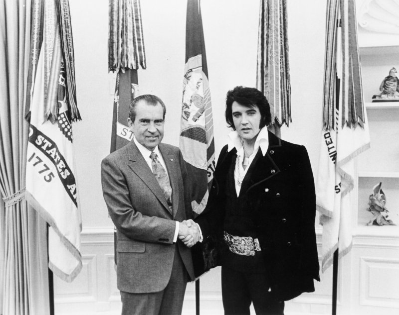
An iconic image

Long Tall Sally

We can treat a grayscale image as a matrix of pixel values. Each pixel has a brightness value between 0 (black) and 1 (white). An 800x600 pixel image can be represented as a matrix with 600 rows and 800 columns, where each entry in the matrix is the brightness value of the corresponding pixel.

# install.packages("imager")

img <- imager::load.image(here("assets", "08-iterate", "elvis-nixon.jpeg"))
str(img)

 'cimg' num [1:800, 1:633, 1, 1] 0.914 0.929 0.91 0.906 0.898 ...

dim(img)

[1] 800 633   1   1

## Long
img_df_long <- as.data.frame(img)

head(img_df_long)

  x y     value
1 1 1 0.9137255
2 2 1 0.9294118
3 3 1 0.9098039
4 4 1 0.9058824
5 5 1 0.8980392
6 6 1 0.8862745

Return to Sender

img_df <- pivot_wider(img_df_long,
                             names_from = y,
                             values_from = value)

dim(img_df)

[1] 800 634

img_df[1:5, 1:5]

# A tibble: 5 × 5
      x   `1`   `2`   `3`   `4`
  <int> <dbl> <dbl> <dbl> <dbl>
1     1 0.914 0.914 0.914 0.910
2     2 0.929 0.929 0.925 0.918
3     3 0.910 0.910 0.902 0.894
4     4 0.906 0.902 0.898 0.894
5     5 0.898 0.894 0.890 0.886

Don’t be Cruel

tmp <- img_df |> select(-x)
dim(tmp)

[1] 800 633

tmp[1:5, 1:5]

# A tibble: 5 × 5
    `1`   `2`   `3`   `4`   `5`
  <dbl> <dbl> <dbl> <dbl> <dbl>
1 0.914 0.914 0.914 0.910 0.902
2 0.929 0.929 0.925 0.918 0.910
3 0.910 0.910 0.902 0.894 0.886
4 0.906 0.902 0.898 0.894 0.890
5 0.898 0.894 0.890 0.886 0.882

# Scaled and centered
tmp_norm <- scale(tmp, center = TRUE, scale = TRUE)
tmp_norm[1:5, 1:5]

             1         2         3         4         5
[1,] 0.3062542 0.3271632 0.3352950 0.3137665 0.2662779
[2,] 0.4172912 0.4326572 0.4124186 0.3645892 0.3165605
[3,] 0.2784949 0.3007897 0.2581714 0.2121212 0.1657127
[4,] 0.2507356 0.2480427 0.2324635 0.2121212 0.1908540
[5,] 0.1952171 0.1952957 0.1810477 0.1612985 0.1405714

# Covariance matrix
cov_mat <- cov(tmp_norm)
dim(cov_mat)

[1] 633 633

cov_mat[1:5, 1:5]

          1         2         3         4         5
1 1.0000000 0.9945150 0.9877773 0.9848553 0.9820028
2 0.9945150 1.0000000 0.9966495 0.9902557 0.9834383
3 0.9877773 0.9966495 1.0000000 0.9958584 0.9866195
4 0.9848553 0.9902557 0.9958584 1.0000000 0.9931752
5 0.9820028 0.9834383 0.9866195 0.9931752 1.0000000

Wooden Heart

Doing the PCA manually, just to show how it works under the hood.

# Decomposition/Factorization into eigenvalues and eigenvectors
cov_eig <- eigen(cov_mat)
names(cov_eig)

[1] "values"  "vectors"

# Eigenvalues (variances)
cov_evals <- cov_eig$values
cov_evals[1:5]

[1] 231.41622 120.60984  56.89806  31.05158  22.82532

# Eigenvectors (principal components)
cov_evecs <- cov_eig$vectors
cov_evecs[1:5, 1:5]

             [,1]        [,2]       [,3]        [,4]       [,5]
[1,] -0.006164854 -0.06573463 0.02875530 -0.03933564 0.06010992
[2,] -0.006734353 -0.06614096 0.02858038 -0.03849782 0.05901673
[3,] -0.007154980 -0.06590388 0.02736392 -0.03892858 0.05852467
[4,] -0.007471463 -0.06604222 0.02671015 -0.03827302 0.05944892
[5,] -0.006484754 -0.06614490 0.02788219 -0.03994717 0.06062967

# Rotation matrix -- ie the coordinates of the
# original data points translated into the
# transformed coordinate space prcomp$rotation
tmp_rot <- tmp_norm %*% cov_evecs
dim(tmp_rot)

[1] 800 633

tmp_rot[1:5, 1:5]

          [,1]      [,2]      [,3]     [,4]     [,5]
[1,] 11.589359 -4.479811 -2.268584 3.666006 4.655793
[2,] 10.917918 -4.386686 -3.477785 4.237974 6.417180
[3,]  9.411595 -4.239953 -4.511044 3.983355 6.585201
[4,]  8.768736 -3.946033 -4.653053 3.398185 4.503424
[5,]  8.452248 -3.153785 -4.491075 2.568274 1.609303

# Should be zero
round(cov(cov_evecs), 2)[1:5,1:5]

     [,1] [,2] [,3] [,4] [,5]
[1,]    0    0    0    0    0
[2,]    0    0    0    0    0
[3,]    0    0    0    0    0
[4,]    0    0    0    0    0
[5,]    0    0    0    0    0

Clean up your own Backyard

But of course we don’t have to do all this manually. R has a built-in function, prcomp(), that does all this for us.

img_pca <- img_df |>
  select(-x) |>
  prcomp(scale = TRUE, center = TRUE)

pca_tidy <- tidy(img_pca, matrix = "pcs")

pca_tidy

# A tibble: 633 × 4
      PC std.dev percent cumulative
   <dbl>   <dbl>   <dbl>      <dbl>
 1     1   15.2   0.366       0.366
 2     2   11.0   0.191       0.556
 3     3    7.54  0.0899      0.646
 4     4    5.57  0.0491      0.695
 5     5    4.78  0.0361      0.731
 6     6    4.56  0.0328      0.764
 7     7    4.06  0.0261      0.790
 8     8    3.66  0.0212      0.811
 9     9    3.37  0.0179      0.829
10    10    3.28  0.0170      0.846
# ℹ 623 more rows

All Shook Up

names(img_pca)

[1] "sdev"     "rotation" "center"   "scale"    "x"       

What are these named things? sdev contains the standard deviations of the principal components. rotation is a matrix where the rows correspond to the columns of the original data, and the columns are the principal components. x is a matrix containing the value of the rotated data multiplied by the rotation matrix. Finally, center and scale are vectors showing the centering and scaling for each observation.

Now, to get from this information back to the original data matrix, we need to multiply x by the transpose of the rotation matrix, and then revert the centering and scaling steps. If we multiply by the transpose of the full rotation matrix (and then un-center and un-scale), we’ll recover the original data matrix exactly. (This is what it means to be able to decompose/factorize the original matrix into these different pieces. Together the pieces can be used to reconstitute the original matrix.)

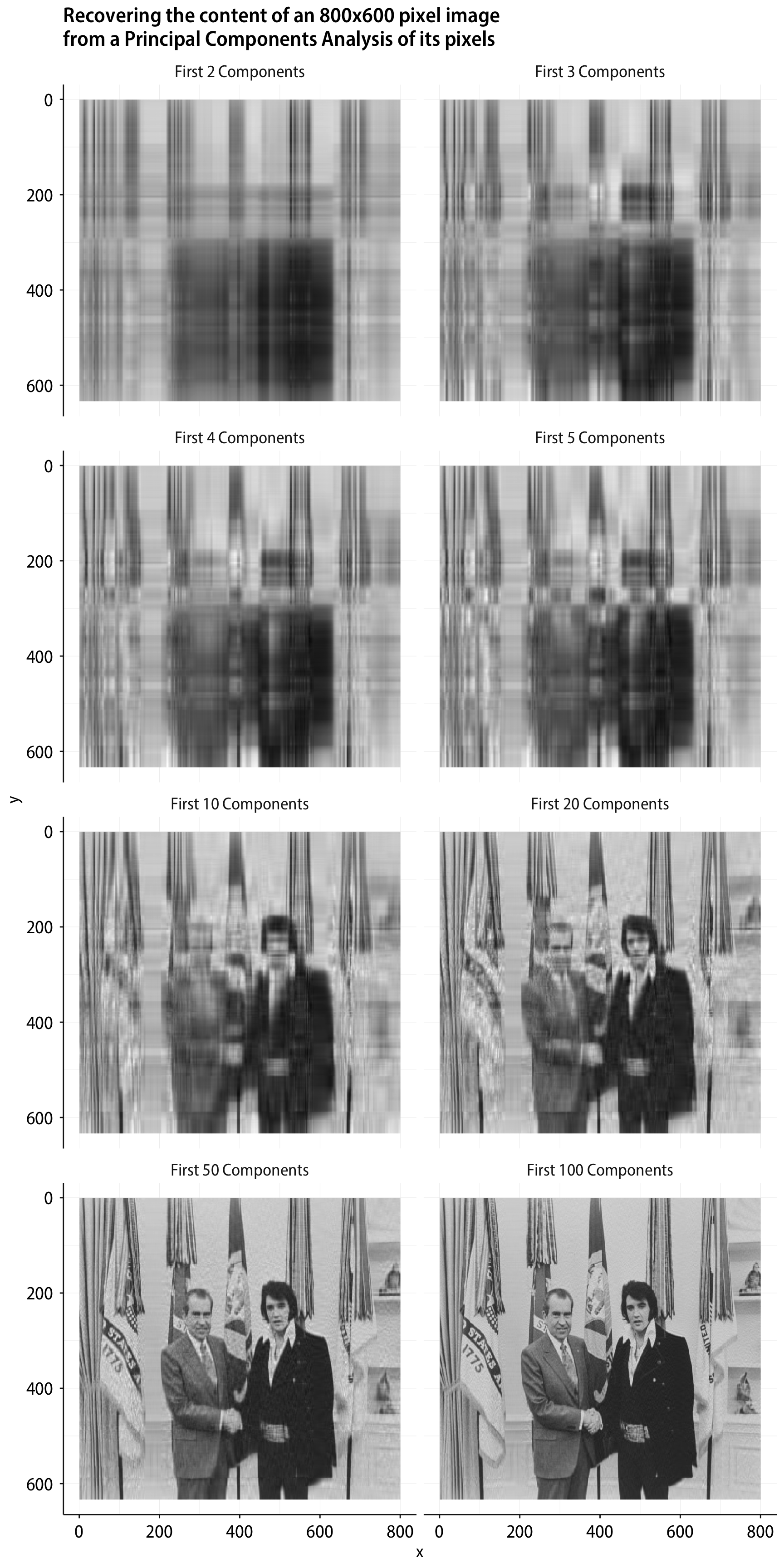
But we can also choose to use just the first few principal components, instead, as we make our way back to something that is the same shape as the original matrix of pixel values. There are 633 components in all (corresponding to the number of rows in the original data matrix), but the scree plot suggests that most of the data is “explained” by a much smaller number of components than that. And so, we can choose to use just the first 2, or 5, or 10, or 20, or 50 components to get back to an approximation of the original data matrix. This is a lossy reconstruction of the original data.

I Gotta Know

Here’s a function that takes a PCA object created by prcomp() and returns an approximation of the original data, calculated by some number (n_comp) of principal components. It returns its results in long format, in a way that mirrors what the Imager library wants. This will make plotting easier in a minute.

reverse_pca <- function(n_comp = 20, pca_object = img_pca){
  ## The pca_object is an object created by base R's prcomp() function.

  ## Multiply the matrix of rotated data by the transpose of the matrix
  ## of eigenvalues (i.e. the component loadings) to get back to a
  ## matrix of original data values
  recon <- pca_object$x[, 1:n_comp] %*% t(pca_object$rotation[, 1:n_comp])

  ## Reverse any scaling and centering that was done by prcomp()

  if(all(pca_object$scale != FALSE)){
    ## Rescale by the reciprocal of the scaling factor, i.e. back to
    ## original range.
    recon <- scale(recon, center = FALSE, scale = 1/pca_object$scale)
  }
  if(all(pca_object$center != FALSE)){
    ## Remove any mean centering by adding the subtracted mean back in
    recon <- scale(recon, scale = FALSE, center = -1 * pca_object$center)
  }

  ## Make it a data frame that we can easily pivot to long format
  ## (because that's the format that the excellent imager library wants
  ## when drawing image plots with ggplot)
  recon_df <- data.frame(cbind(1:nrow(recon), recon))
  colnames(recon_df) <- c("x", 1:(ncol(recon_df)-1))

  ## Return the data to long form
  recon_df_long <- recon_df |>
    tidyr::pivot_longer(cols = -x,
                        names_to = "y",
                        values_to = "value") |>
    mutate(y = as.numeric(y)) |>
    arrange(y) |>
    as.data.frame()

  tibble::as_tibble(recon_df_long)
}

It’s Now or Never

## The sequence of PCA components we want
n_pcs <- c(2:5, 10, 20, 50, 100)
names(n_pcs) <- paste("First", n_pcs, "Components", sep = "_")

## Map reverse_pca()
recovered_imgs <- map(n_pcs, reverse_pca) |>
  list_rbind(names_to = "pcs") |>
  mutate(pcs = str_replace_all(pcs, "_", " "),
         pcs = factor(pcs, levels = unique(pcs), ordered = TRUE))

recovered_imgs

# A tibble: 4,051,200 × 4
   pcs                    x     y value
   <ord>              <dbl> <dbl> <dbl>
 1 First 2 Components     1     1 0.902
 2 First 2 Components     2     1 0.902
 3 First 2 Components     3     1 0.902
 4 First 2 Components     4     1 0.899
 5 First 2 Components     5     1 0.892
 6 First 2 Components     6     1 0.886
 7 First 2 Components     7     1 0.877
 8 First 2 Components     8     1 0.858
 9 First 2 Components     9     1 0.823
10 First 2 Components    10     1 0.772
# ℹ 4,051,190 more rows

Jailhouse Rock

ggplot(data = recovered_imgs,
            mapping = aes(x = x, y = y, fill = value)) +
  geom_raster() +
  scale_y_reverse() +
  scale_fill_gradient(low = "black", high = "white") +
  facet_wrap(~ pcs, ncol = 2) +
  guides(fill = "none") +
  labs(title = "Recovering the content of an 800x600 pixel image\nfrom a Principal Components Analysis of its pixels") +
  theme(strip.text = element_text(face = "bold", size = rel(1.2)),
        plot.title = element_text(size = rel(1.5)))