── Attaching core tidyverse packages ──────────────────────── tidyverse 2.0.0 ──
✔ dplyr     1.1.4     ✔ readr     2.1.5
✔ forcats   1.0.0     ✔ stringr   1.5.1
✔ ggplot2   3.5.1     ✔ tibble    3.2.1
✔ lubridate 1.9.3     ✔ tidyr     1.3.1
✔ purrr     1.0.2
── Conflicts ────────────────────────────────────────── tidyverse_conflicts() ──
✖ dplyr::filter() masks stats::filter()
✖ dplyr::lag()    masks stats::lag()
ℹ Use the conflicted package (<http://conflicted.r-lib.org/>) to force all conflicts to become errors
here() starts at /Users/kjhealy/Documents/courses/mptc

Loading required package: sysfonts

Loading required package: showtextdbExample 11: Visualizing Data
library(tidyverse)
library(scales)
Attaching package: 'scales'The following object is masked from 'package:purrr':
discardThe following object is masked from 'package:readr':
col_factorlibrary(here)
library(socviz)
my_colors <- ggokabeito::palette_okabe_ito()Census Data Example
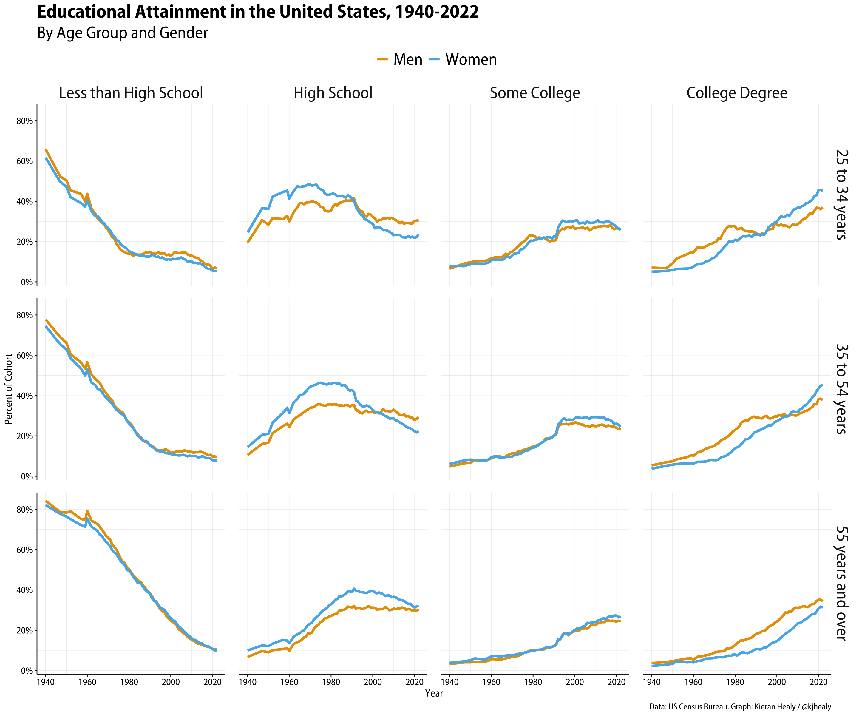
A faceted view of some multi-way data.
attainment_levs <- c("Less than High School",
                     "High School",
                     "Some College",
                     "College Degree")

edage_df <- read_csv(here("files", "examples", "census_edage.csv")) |>
  # Need to order the Education categories
  mutate(attainment = factor(attainment,
                             levels = attainment_levs,
                             ordered = TRUE))
Rows: 4824 Columns: 6
── Column specification ────────────────────────────────────────────────────────
Delimiter: ","
chr (3): group, level, attainment
dbl (3): year, total, count
ℹ Use `spec()` to retrieve the full column specification for this data.
ℹ Specify the column types or set `show_col_types = FALSE` to quiet this message.edage_df# A tibble: 4,824 × 6
group year total level attainment count
<chr> <dbl> <dbl> <chr> <ord> <dbl>
1 25 Years and Over, Both Sexes 2022 226274 Elementary: 0 to… Less than… 2203
2 25 Years and Over, Both Sexes 2022 226274 Elementary: 5 to… Less than… 5732
3 25 Years and Over, Both Sexes 2022 226274 High School: 1 t… Less than… 11998
4 25 Years and Over, Both Sexes 2022 226274 High School: 4 y… High Scho… 64465
5 25 Years and Over, Both Sexes 2022 226274 College: 1 to 3 … Some Coll… 56659
6 25 Years and Over, Both Sexes 2022 226274 College: 4 years… College D… 85217
7 25 Years and Over, Both Sexes 2021 224580 Elementary: 0 to… Less than… 2074
8 25 Years and Over, Both Sexes 2021 224580 Elementary: 5 to… Less than… 5862
9 25 Years and Over, Both Sexes 2021 224580 High School: 1 t… Less than… 12118
10 25 Years and Over, Both Sexes 2021 224580 High School: 4 y… High Scho… 62547
# ℹ 4,814 more rowsThis data is not tidy.
unique(edage_df$group) [1] "25 Years and Over, Both Sexes" "25 Years and Over, Male"
[3] "25 Years and Over, Female" "25 to 34 Years, Both Sexes"
[5] "25 to 34 Years, Male" "25 to 34 Years, Female"
[7] "35 to 54 Years, Both Sexes" "35 to 54 Years, Male"
[9] "35 to 54 Years, Female" "55 Years and Over, Both Sexes"
[11] "55 Years and Over, Male" "55 Years and Over, Female" We’re going to filter to what we need and graph it.
edage_coarse_df <- edage_df |>
  group_by(group, year, attainment) |>
  summarize(total = mean(total),
            count = sum(count)) |>
  mutate(prop = count/total) |>
  separate_wider_delim(group, delim = ",", names = c("age", "sex")) |>
  mutate(sex = str_squish(sex))
`summarise()` has grouped output by 'group', 'year'. You can override using the
`.groups` argument.edage_coarse_df# A tibble: 3,216 × 7
# Groups: year [67]
age sex year attainment total count prop
<chr> <chr> <dbl> <ord> <dbl> <dbl> <dbl>
1 25 Years and Over Both Sexes 1940 Less than High School 74776 55700 0.745
2 25 Years and Over Both Sexes 1940 High School 74776 10552 0.141
3 25 Years and Over Both Sexes 1940 Some College 74776 4075 0.0545
4 25 Years and Over Both Sexes 1940 College Degree 74776 3407 0.0456
5 25 Years and Over Both Sexes 1947 Less than High School 82578 54406 0.659
6 25 Years and Over Both Sexes 1947 High School 82578 16926 0.205
7 25 Years and Over Both Sexes 1947 Some College 82578 5533 0.0670
8 25 Years and Over Both Sexes 1947 College Degree 82578 4424 0.0536
9 25 Years and Over Both Sexes 1950 Less than High School 87484 55925 0.639
10 25 Years and Over Both Sexes 1950 High School 87484 17625 0.201
# ℹ 3,206 more rowsStill not tidy!
unique(edage_coarse_df$age)[1] "25 Years and Over" "25 to 34 Years" "35 to 54 Years"
[4] "55 Years and Over"Final pre-plot data:
plot_df <- edage_coarse_df |>
  filter(sex != "Both Sexes", age != "25 Years and Over") |>
  mutate(gender = case_match(sex,
                             "Male" ~ "Men",
                             "Female" ~ "Women")) |>
  mutate(age = str_to_lower(age))

plot_df
# A tibble: 1,608 × 8
# Groups: year [67]
age sex year attainment total count prop gender
<chr> <chr> <dbl> <ord> <dbl> <dbl> <dbl> <chr>
1 25 to 34 years Female 1940 Less than High School 10818 6675 0.617 Women
2 25 to 34 years Female 1940 High School 10818 2653 0.245 Women
3 25 to 34 years Female 1940 Some College 10818 862 0.0797 Women
4 25 to 34 years Female 1940 College Degree 10818 544 0.0503 Women
5 25 to 34 years Female 1947 Less than High School 11733 5832 0.497 Women
6 25 to 34 years Female 1947 High School 11733 4293 0.366 Women
7 25 to 34 years Female 1947 Some College 11733 915 0.0780 Women
8 25 to 34 years Female 1947 College Degree 11733 640 0.0545 Women
9 25 to 34 years Female 1950 Less than High School 12172 5743 0.472 Women
10 25 to 34 years Female 1950 High School 12172 4410 0.362 Women
# ℹ 1,598 more rowsAnd off we go:
plot_df |>
  ggplot(aes(x = year, y = prop, color = gender)) +
  geom_line(linewidth = 1.5) +
  facet_grid(age ~ attainment) +
  scale_y_continuous(labels = label_percent()) +
  scale_color_manual(values = my_colors) +
  labs(x = "Year",
       y = "Percent of Cohort",
       color = "",
       title = "Educational Attainment in the United States, 1940-2022",
       subtitle = "By Age Group and Gender",
       caption = "Data: US Census Bureau. Graph: Kieran Healy / @kjhealy") +
  theme(panel.spacing.x = unit(1.2, "lines"),
        panel.spacing.y = unit(1.1, "lines"),
        strip.text = element_text(size = rel(1.8)),
        plot.title = element_text(size = rel(2)),
        plot.subtitle = element_text(size = rel(1.8)),
        legend.text = element_text(size = rel(1.8)))